You've taken a couple of big steps so far by covering vectors and linear transformations, but you're not truly a big stepper until you understand dot products. Let's start with the standard introduction, then dig into why the computation actually works.
Numerical Method
The dot product takes two vectors of the same dimension (two lists of numbers with the same length), pairs up the coordinates, multiplies each pair, and adds the results.

The dot product pairs up coordinates, multiplies them, and adds the results
Here's what that looks like with two 2D vectors:
Geometric Interpretation
The dot product also has a clean geometric interpretation. Given two vectors $\mathbf{v}$ and $\mathbf{w}$, imagine projecting $\mathbf{w}$ onto the line passing through the origin and the tip of $\mathbf{v}$.

Projecting $\mathbf{w}$ onto the line defined by $\mathbf{v}$
Multiply the length of that projection by the length of $\mathbf{v}$, and that's your dot product $(\mathbf{v} \cdot \mathbf{w})$.

The dot product equals (length of projection) × (length of $\mathbf{v}$)
When the projection of $\mathbf{w}$ points in the opposite direction of $\mathbf{v}$, the dot product is negative.

When the projection points opposite to $\mathbf{v}$, the dot product is negative
Essentially, the sign of the dot product tells you how aligned two given vectors are:
- $\mathbf{v} \cdot \mathbf{w} > 0$ → they point in similar directions
- $\mathbf{v} \cdot \mathbf{w} = 0$ → they are perpendicular (the projection of one onto the other is the zero vector)
- $\mathbf{v} \cdot \mathbf{w} < 0$ → they point in opposing directions

The sign of the dot product indicates directional alignment
Order Doesn't Matter
The geometric picture looks asymmetric as it treats the two vectors very differently. But the dot product is commutative. You could project $\mathbf{v}$ onto $\mathbf{w}$ instead, multiply by the length of $\mathbf{w}$, and get the same answer.

Even though this feels like a very different process, it produces the same result
When $\mathbf{v}$ and $\mathbf{w}$ have the same length, the symmetry is obvious. Projecting $\mathbf{w}$ onto $\mathbf{v}$ is a mirror image of projecting $\mathbf{v}$ onto $\mathbf{w}$.

Equal-length vectors have perfect symmetry
If you scale $\mathbf{v}$ by some constant (say $2$), the symmetry breaks, but the dot product still doubles either way. Think of it as doubling the length of the vector you project onto, or as doubling the projection itself. Either interpretation gives you $2(\mathbf{v} \cdot \mathbf{w})$.

The length of projecting $\mathbf{w}$ onto $2\mathbf{v}$ stays the same, while the length of $2\mathbf{v}$ doubles

The length of projecting $2\mathbf{v}$ onto $\mathbf{w}$ doubles, while the length of $\mathbf{w}$ stays the same
OK, that's great and all, but what does this numerical process have to do with geometric projection? To answer that properly, we need to talk about linear transformations from 2D to 1D.

Functions that take in 2D vectors and spit out numbers
Linear Transformations
These are functions that take in 2D vectors and output single numbers. Because they're linear, they're far more constrained than arbitrary functions with 2D inputs and 1D outputs.
Rather than get into formal definitions of linearity, let's focus on an equivalent visual property: if you take a line of evenly spaced dots and apply a linear transformation, the dots stay evenly spaced in the output.

A line of evenly spaced dots remains evenly spaced in the output
If the dots come out unevenly spaced, the transformation isn't linear.
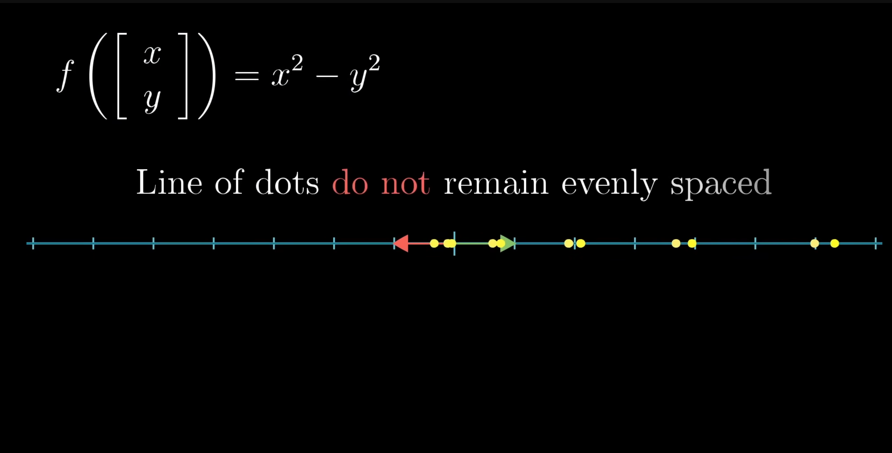
A non-linear transformation produces unevenly spaced output
Just like in higher dimensions, a linear transformation from 2D to 1D is completely determined by where $\hat{\imath}$ and $\hat{\jmath}$ land. Since each one lands on a single number, the whole transformation is described by a $1 \times 2$ matrix.

This linear transformation is described by a $1 \times 2$ matrix
Say a linear transformation takes $\hat{\imath}$ to $2$ and $\hat{\jmath}$ to $-1$. Where does $\begin{bmatrix} 3 \\ 2 \end{bmatrix}$ end up? First, let's break it into its basis components: $3\hat{\imath} + 2\hat{\jmath}$.

Breaking a vector into its basis components
Linearity tells us:

Following where the scaled basis vectors land under the transformation
This calculation is called matrix-vector multiplication, and it's computationally identical to a dot product.

$1 \times 2$ matrix-vector multiplication is computationally identical to a dot product
There's a natural correspondence here: every $1 \times 2$ matrix has an associated 2D vector. Just tilt the vector on its side to get the matrix, or tip the matrix back up to get the vector.

There is a nice association between $1 \times 2$ matrices and 2D vectors
Numerically, that might seem trivial, but it's quite significant from the geometric perspective. This empirically proves that there's a connection between linear transformations that output numbers and vectors themselves.

Visual representation of the connection between linear transformations to numbers and 2D vectors
Unit Vector
To help you visualize unit vectors, place a copy of the number line diagonally in 2D space with $0$ at the origin. Let $\hat{\mathbf{u}}$ be the unit vector pointing to $1$ on this line.

A diagonal number line with unit vector $\hat{\mathbf{u}}$ pointing to $1$
Projecting 2D vectors onto this diagonal line defines a function from 2D vectors to numbers.

Some example vectors

The example vectors projected onto the line defined by $\hat{\mathbf{u}}$
This projection function is linear, and since it maps 2D to 1D, some $1 \times 2$ matrix describes it. To find that matrix, we need to figure out where $\hat{\imath}$ and $\hat{\jmath}$ land.

Some $1 \times 2$ matrix describes this projection

Where $\hat{\imath}$ and $\hat{\jmath}$ land when projected
Here's where things get interesting (relatively speaking). Both $\hat{\imath}$ and $\hat{\mathbf{u}}$ are unit vectors, so projecting $\hat{\imath}$ onto $\hat{\mathbf{u}}$'s line is perfectly symmetrical to projecting $\hat{\mathbf{u}}$ onto the x-axis. That means $\hat{\imath}$ lands at the x-coordinate of $\hat{\mathbf{u}}$.

The projection of $\hat{\imath}$ onto $\hat{\mathbf{u}}$'s line is symmetric to projecting $\hat{\mathbf{u}}$ onto the x-axis

$\hat{\imath}$ lands at the x-coordinate of $\hat{\mathbf{u}}$
Same reasoning: $\hat{\jmath}$ lands at the y-coordinate of $\hat{\mathbf{u}}$.

$\hat{\jmath}$ lands at the y-coordinate of $\hat{\mathbf{u}}$
So the $1 \times 2$ matrix describing this projection is just the coordinates of $\hat{\mathbf{u}}$. Multiplying any vector by this matrix is the same as dotting with $\hat{\mathbf{u}}$.

The projection transformation matrix contains the coordinates of $\hat{\mathbf{u}}$

Matrix-vector multiplication is computationally identical to a dot product with $\hat{\mathbf{u}}$
That's why dotting with a unit vector gives you the projection onto that vector's span. The vector is really just a linear transformation in disguise.

The dot product with a unit vector is projection onto that vector's span
What about non-unit vectors? Scale $\hat{\mathbf{u}}$ by $3$, and each component triples, so the associated matrix scales by $3$ too.

Scaling $\hat{\mathbf{u}}$ by a factor of $3$

The associated transformation matrix scales accordingly
The new transformation still projects onto the same line, but then scales the result by $3$. Just like with non-unit vectors, the dot product here is just a matter of projecting, then scaling.

Project onto the number line, then scale by $3$
Duality
Alright, we just covered some pretty esoteric stuff. Let's zoom out and recap a bit before wrapping up. We started with the geometric operation of projecting 2D space onto a diagonal number line. Because it was linear, a $1 \times 2$ matrix had to describe it. And since multiplying by a $1 \times 2$ matrix is the same as a dot product, the transformation was inescapably tied to a specific 2D vector.

A linear transformation defined geometrically by projecting onto a diagonal number line

The transformation is inescapably related to some 2D vector
This means that any linear transformation whose output space is the number line corresponds to a unique vector $\vec{\mathbf{v}}$, such that applying the transformation to $\vec{\mathbf{w}}$ is the same as computing $\vec{\mathbf{v}} \cdot \vec{\mathbf{w}}$. This correspondence is called duality.
Duality shows up everywhere in math. Put simply, it's a natural-but-surprising correspondence between two types of mathematical objects.
Conclusion
On the surface, the dot product is a geometric tool for measuring how much two vectors align. Under the surface, it's a bridge between vectors and linear transformations. Every vector secretly encodes a transformation from its space down to the number line.