Last chapter we walked through the internals of a transformer. Now let's focus on the mechanism that makes the whole thing work: attention. The name comes from the 2017 paper "Attention Is All You Need," and the title is barely an exaggeration.
Attention
Motivating Examples
Consider these three phrases: American shrew mole, One mole of carbon dioxide, and Take a biopsy of the mole. The word "mole" means something different each time, yet after the initial embedding step the vector for "mole" would be identical in all three cases. The embedding is just a lookup table with no awareness of context.
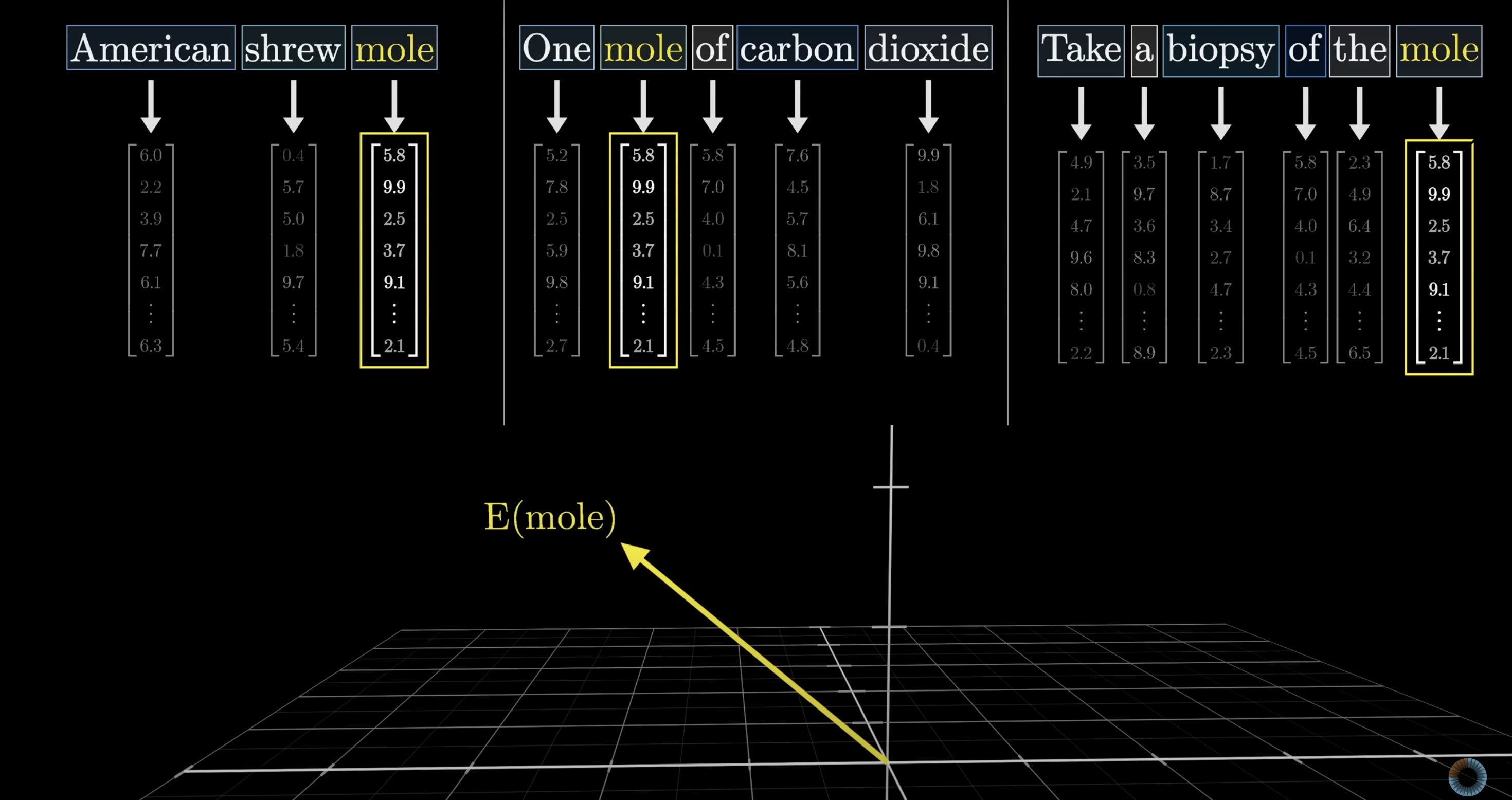
The same token can mean very different things depending on context
That's where attention comes in. The attention block lets surrounding embeddings pass information into the "mole" vector, nudging it toward the right meaning. A well-trained model will have learned distinct directions in the embedding space for each sense of the word.
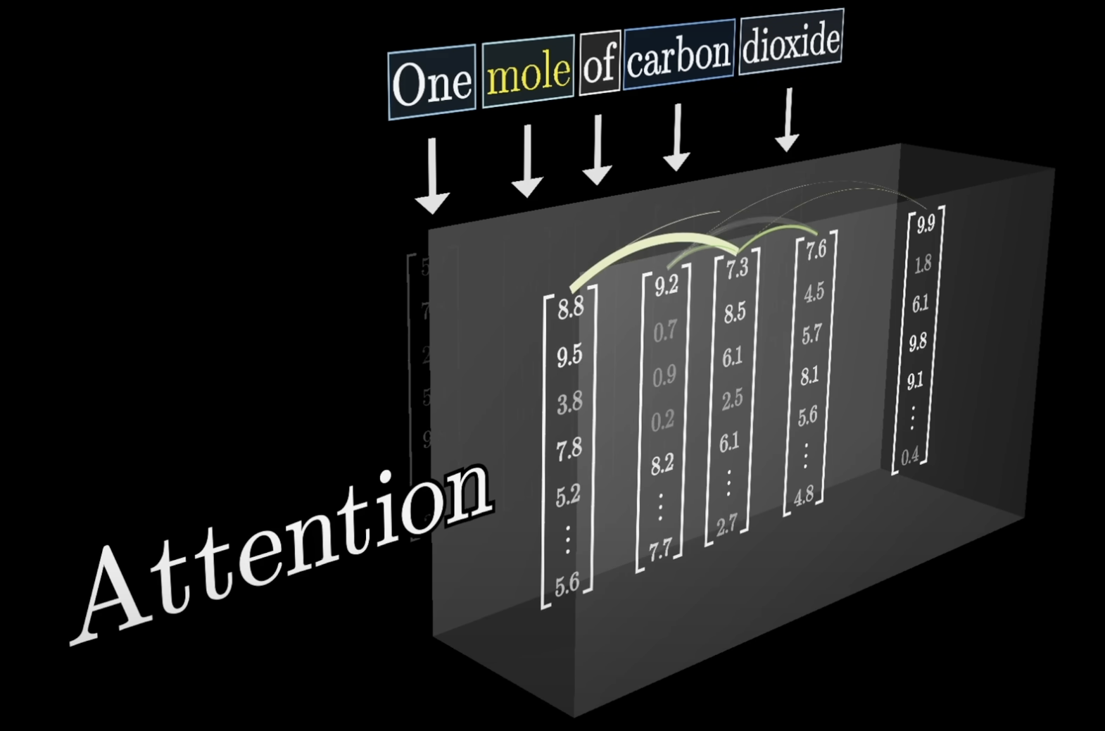
Attention lets surrounding words update a token's embedding
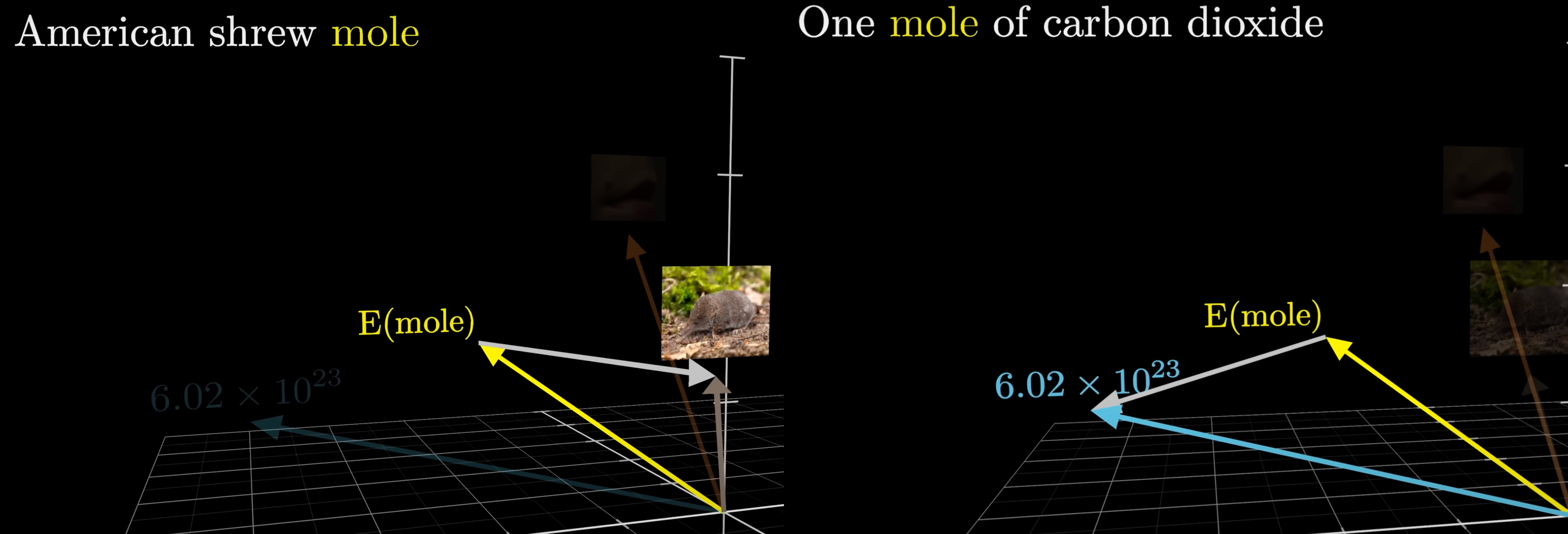
Attention adds a context-dependent adjustment to the generic embedding
Same idea with "tower." The generic embedding doesn't know if we mean the Eiffel Tower or a miniature chess piece. Context like "Eiffel" should push the vector toward Paris and iron; adding "miniature" should pull it away from tall and large.
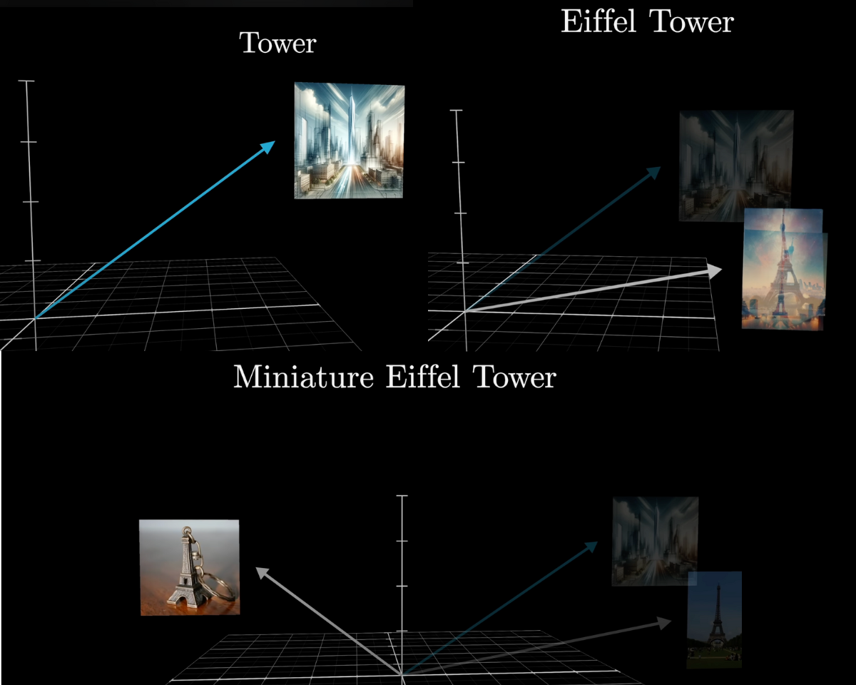
Context like "Eiffel" or "miniature" refines what "tower" means
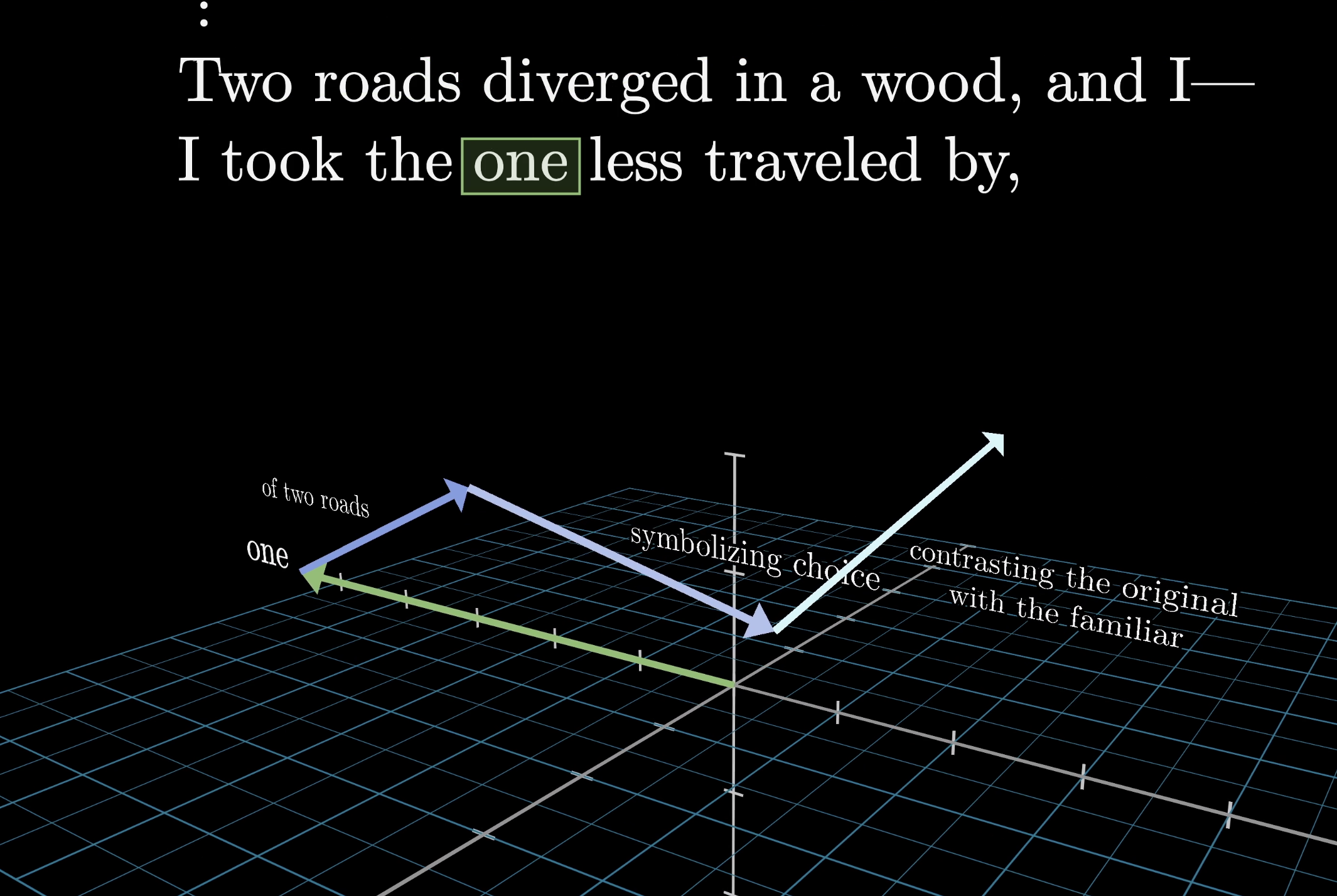
Attention can move information across long distances. Remember, only the last vector in the sequence drives next-token prediction. If the input is an entire mystery novel ending with "Therefore the murderer was…", that final vector needs to encode everything relevant from the full context window.
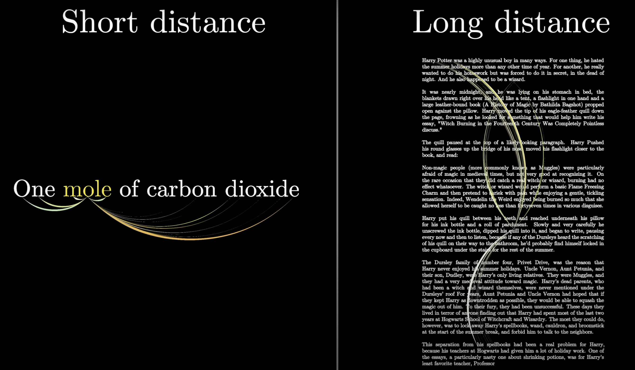
Attention can move information across large distances
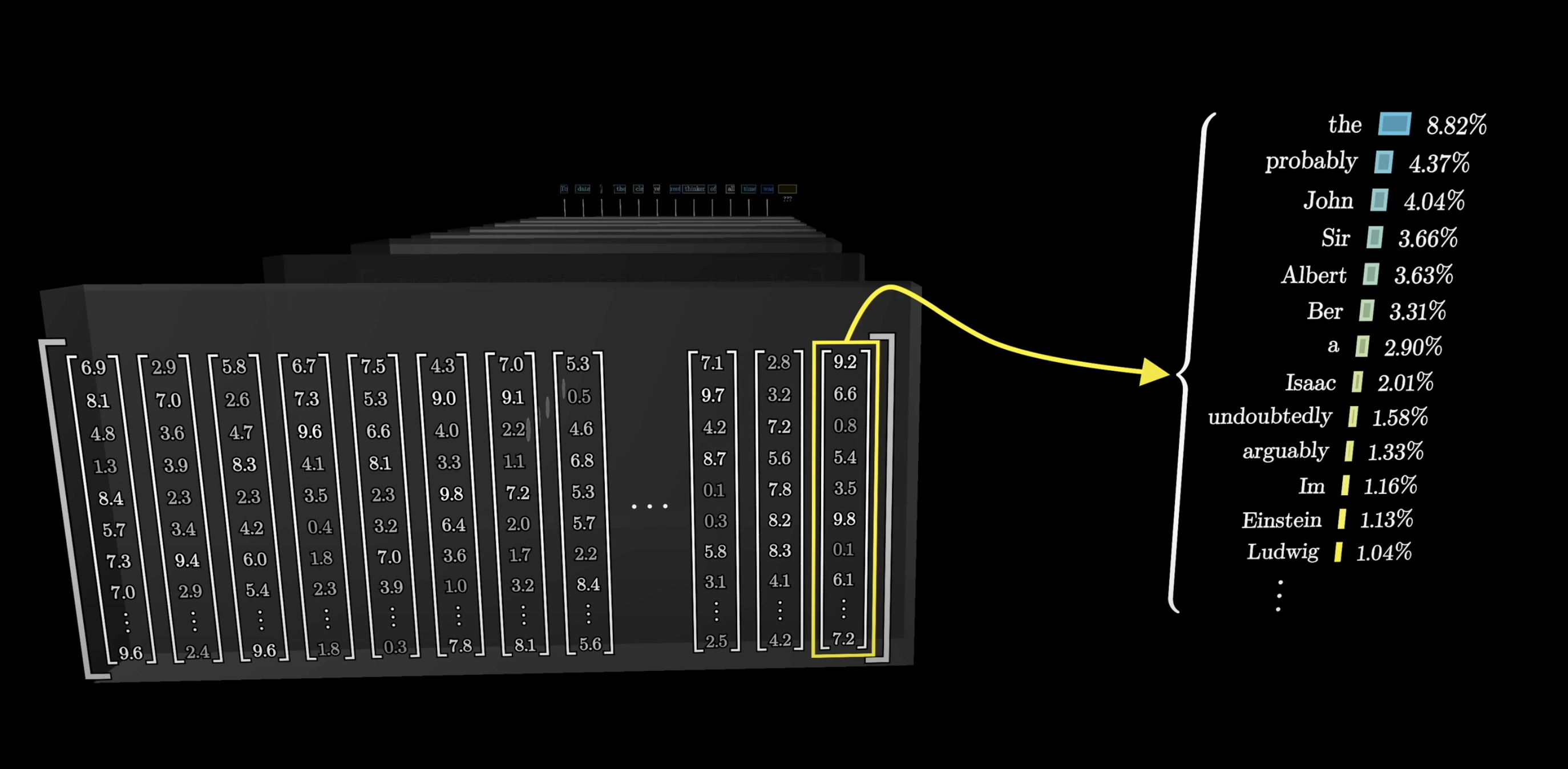
The final position is what drives next-token prediction
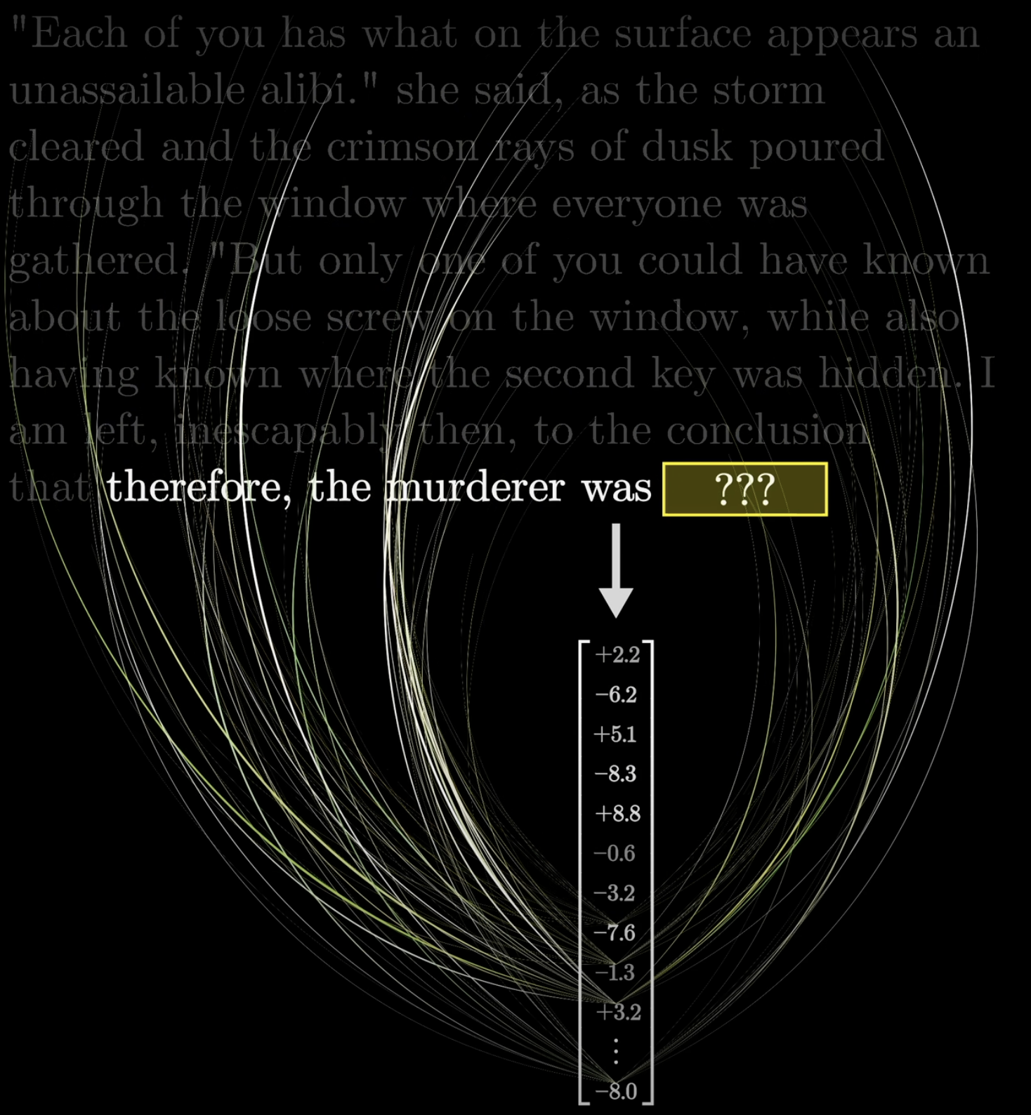
The last vector must contain everything relevant for prediction
The Attention Pattern
We'll start with a single head of attention. Later we'll see how the full attention block runs many heads in parallel.
A single attention head produces an attention pattern
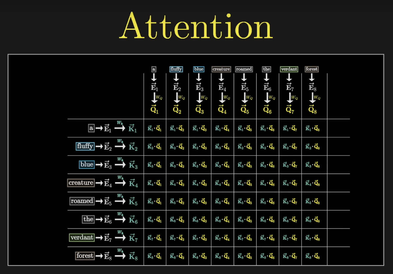
To keep things concrete, our input is: "A fluffy blue creature roamed the verdant forest." For now, the only update we care about is adjectives adjusting the embeddings of their corresponding nouns.
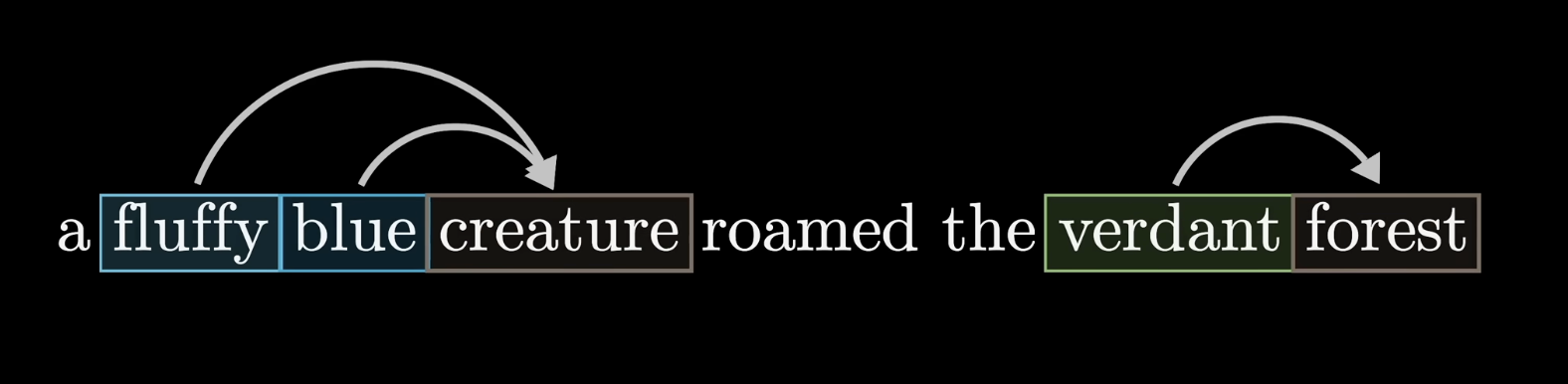
Toy intuition: adjectives push context into their nouns
Each word starts as a high-dimensional embedding vector $\vec{E}$ that also encodes position. Our goal: produce refined embeddings $\vec{E}'$ where the nouns have absorbed meaning from their adjectives.
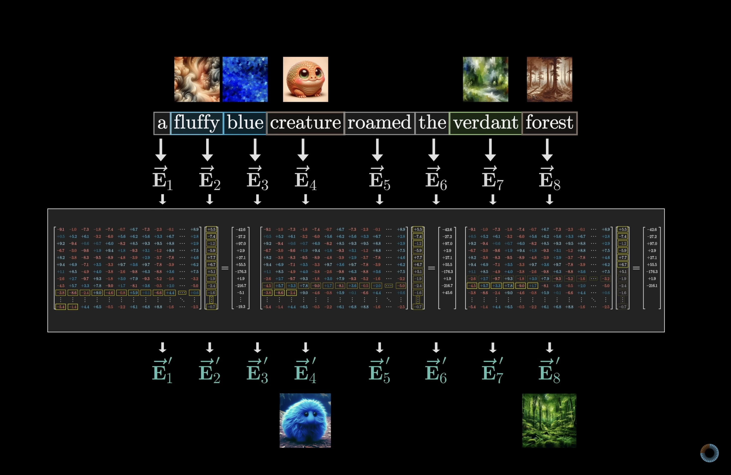
Each token starts as an embedding vector $\vec{E}$
Queries
Each token produces a query vector, conceptually asking: "What am I looking for in the surrounding context?"
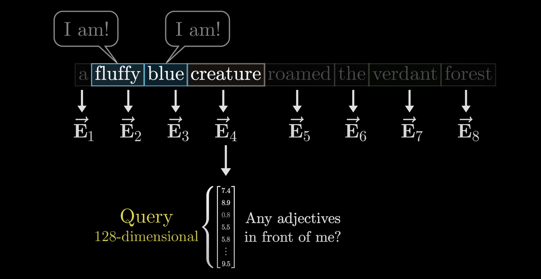
Each token poses a query about what context it needs
Computing a query means multiplying a learned matrix $W_Q$ by the embedding. The query lives in a much smaller space than the embedding itself.
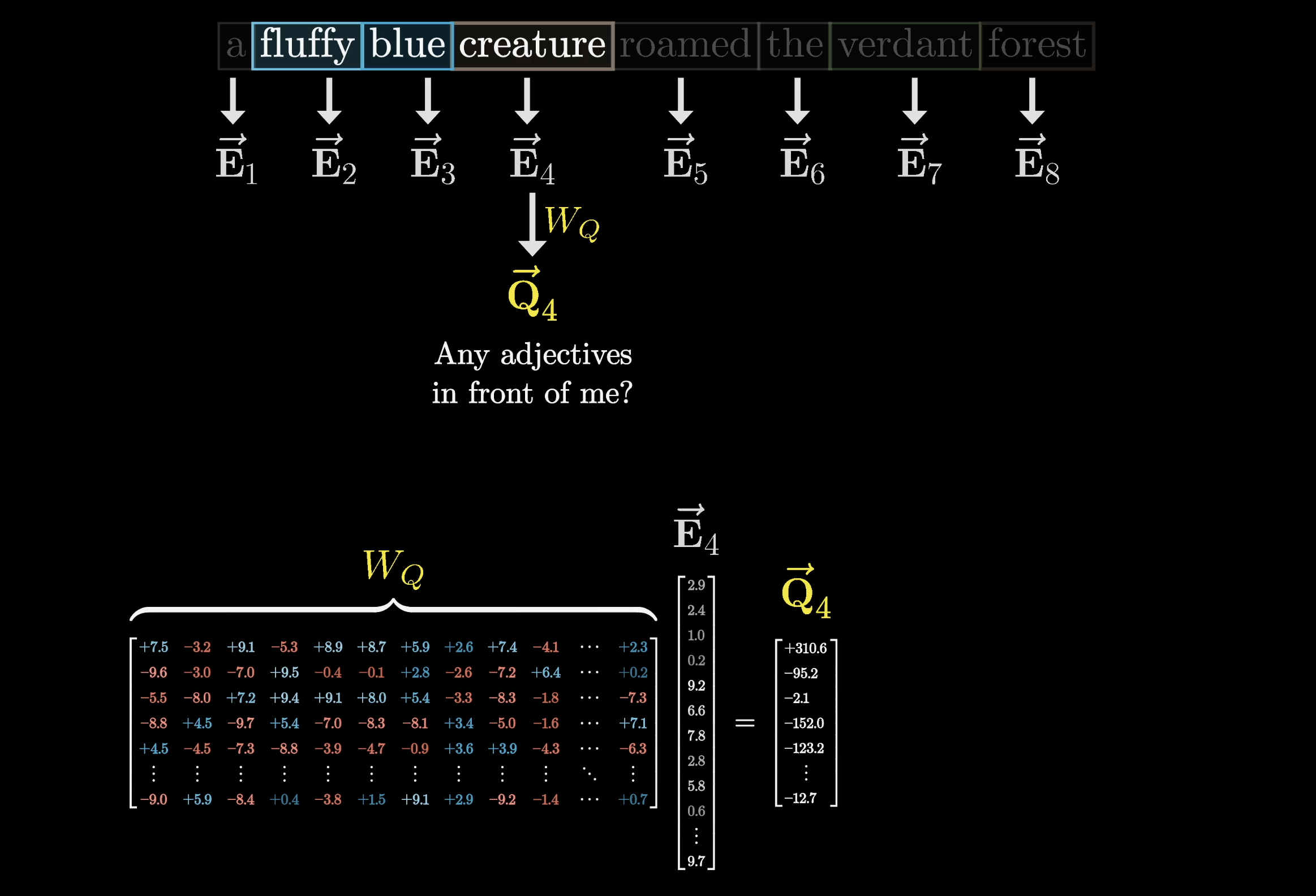
$W_Q$ maps each embedding into a smaller query space
$W_Q$ is applied to every embedding in the context, one query per token. In our toy example, think of it as mapping noun embeddings to a direction that encodes "looking for adjectives in preceding positions."
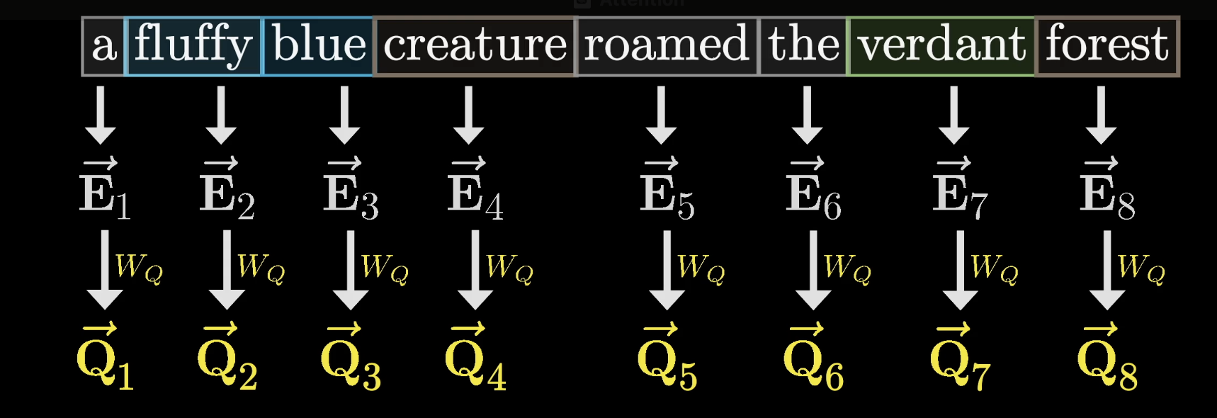
Every token gets its own query
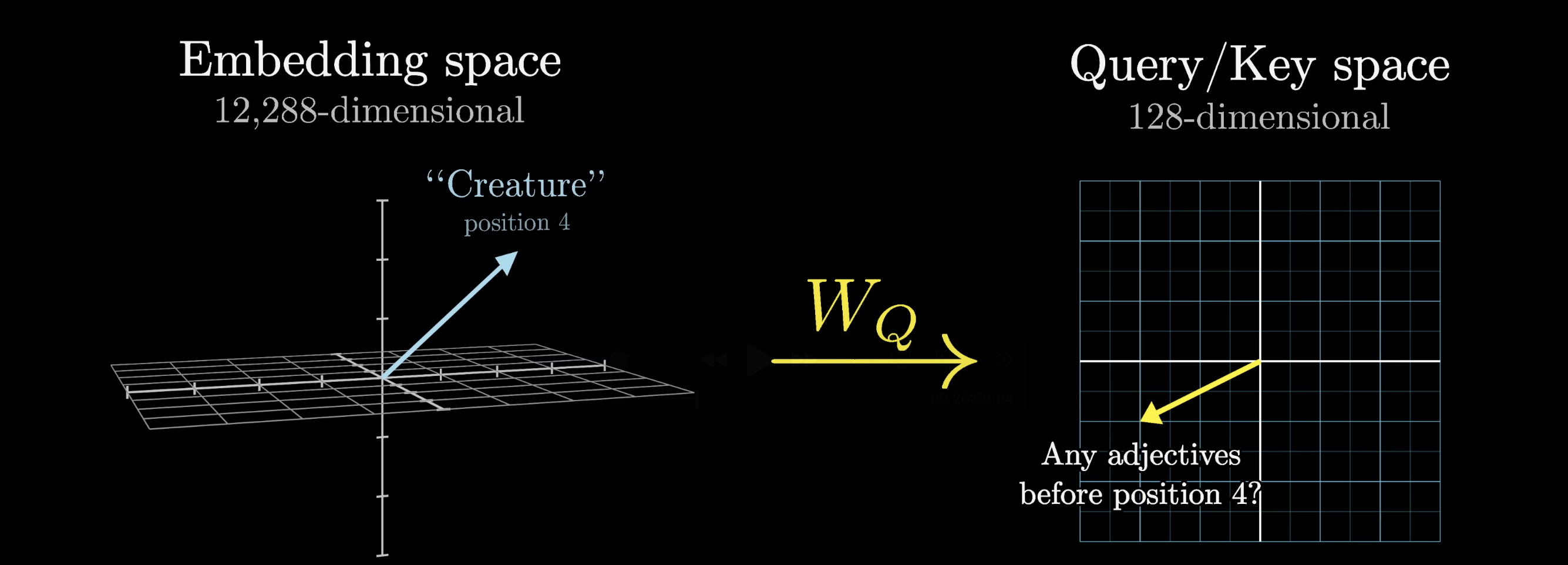
The query space captures what each token is searching for
Keys
At the same time, a second learned matrix, the key matrix ($W_K$), maps each embedding to a key vector. Think of keys as potential answers to the queries.
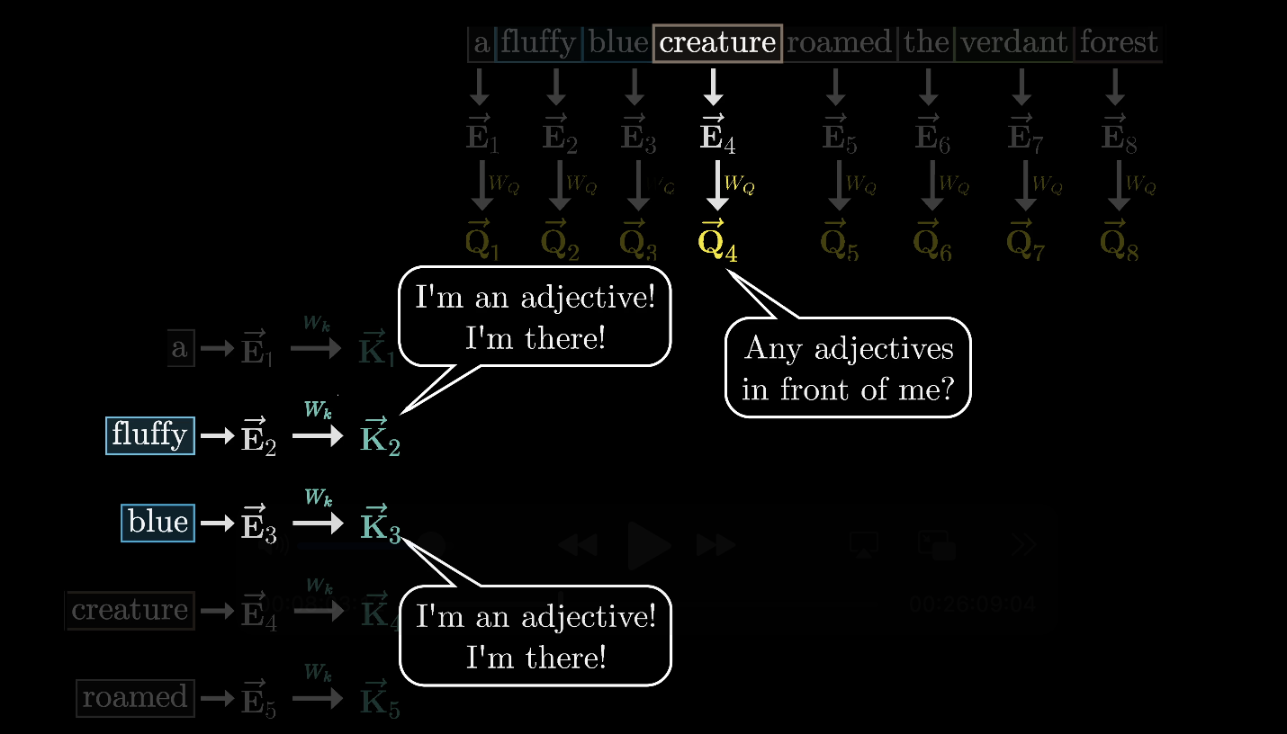
$W_K$ maps each embedding to a key vector
We want keys to match queries when they closely align. In our example, the key matrix maps adjectives like "fluffy" and "blue" to vectors closely aligned with the query from "creature."
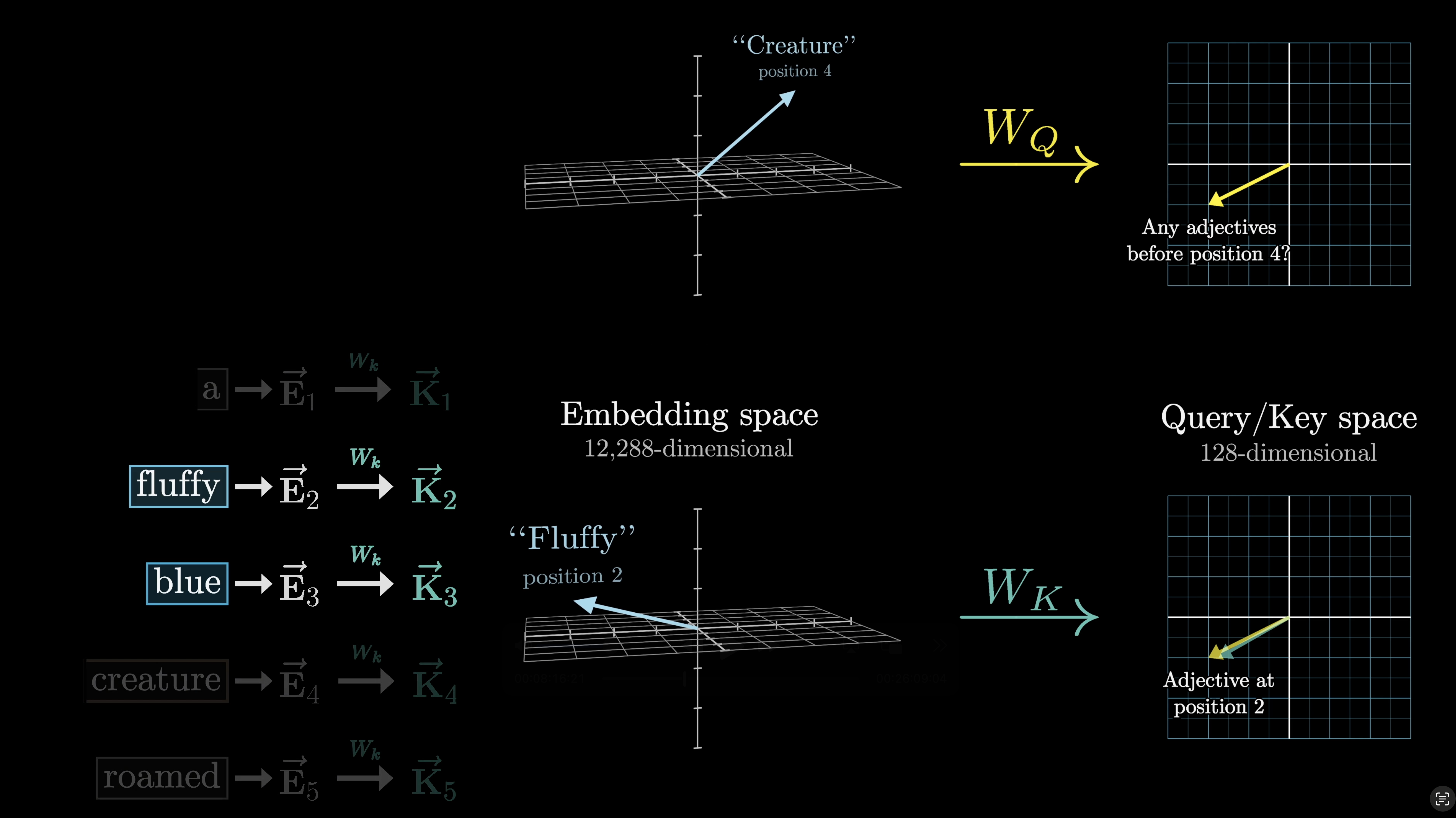
Strong alignment between a key and query indicates relevance
Dot Products Create Relevance Scores
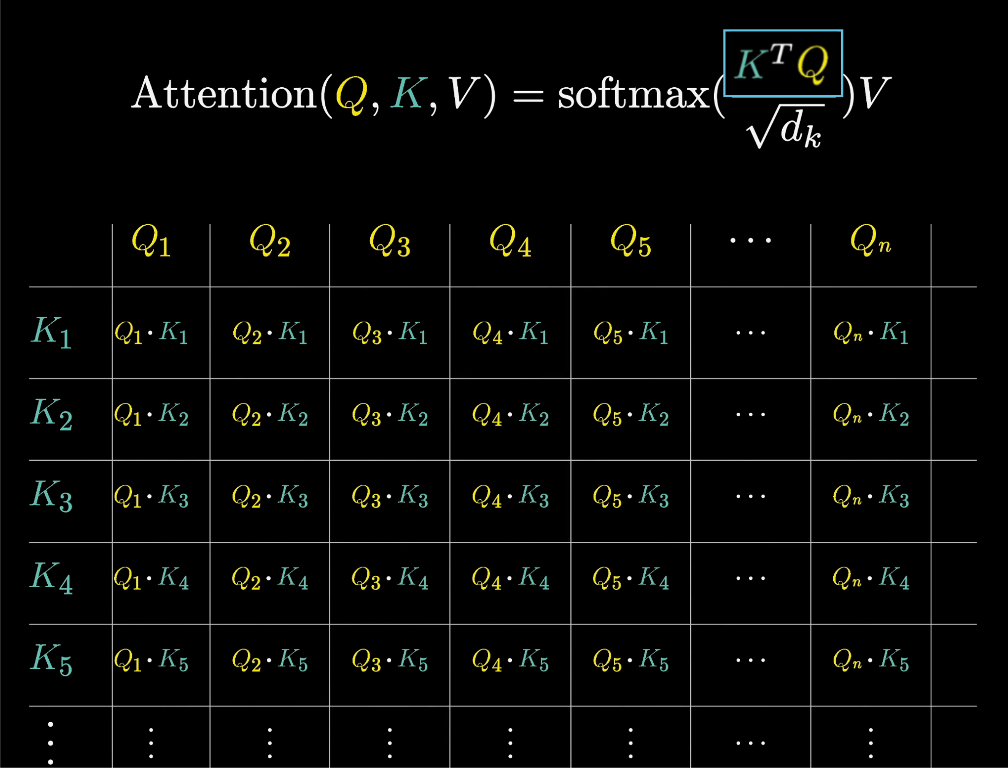
For each query-key pair we compute a dot product. Larger dot product = stronger alignment = higher relevance.
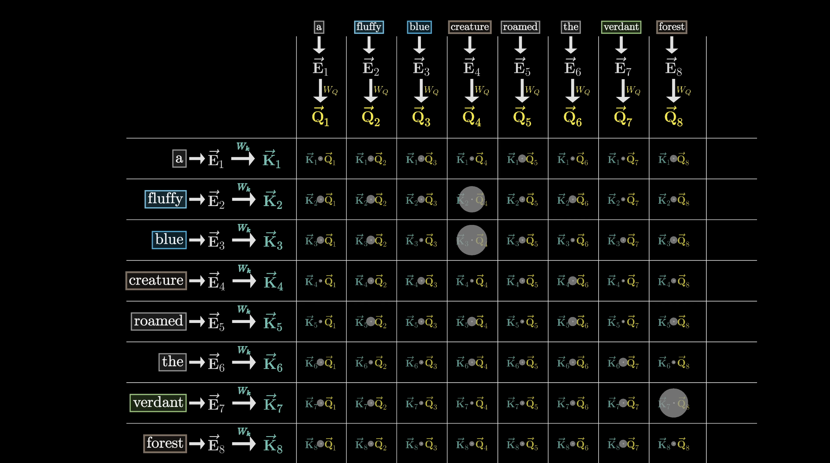
Bigger dots = larger dot products = stronger attention
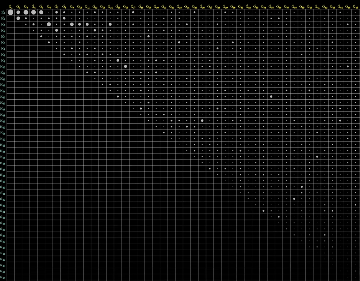
Computing all the dot products gives us a grid of raw scores showing how relevant each word is to updating every other word.
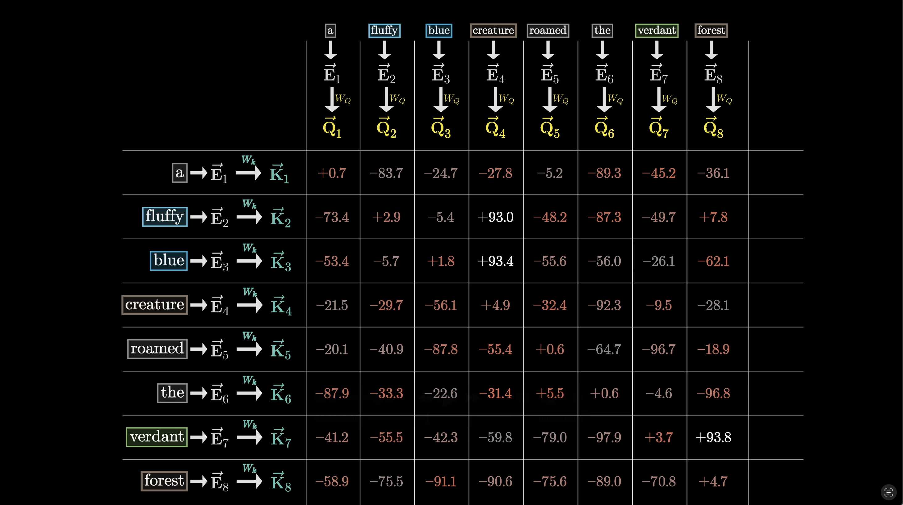
A score matrix: how much each position attends to every other
Softmax Turns Scores into Weights
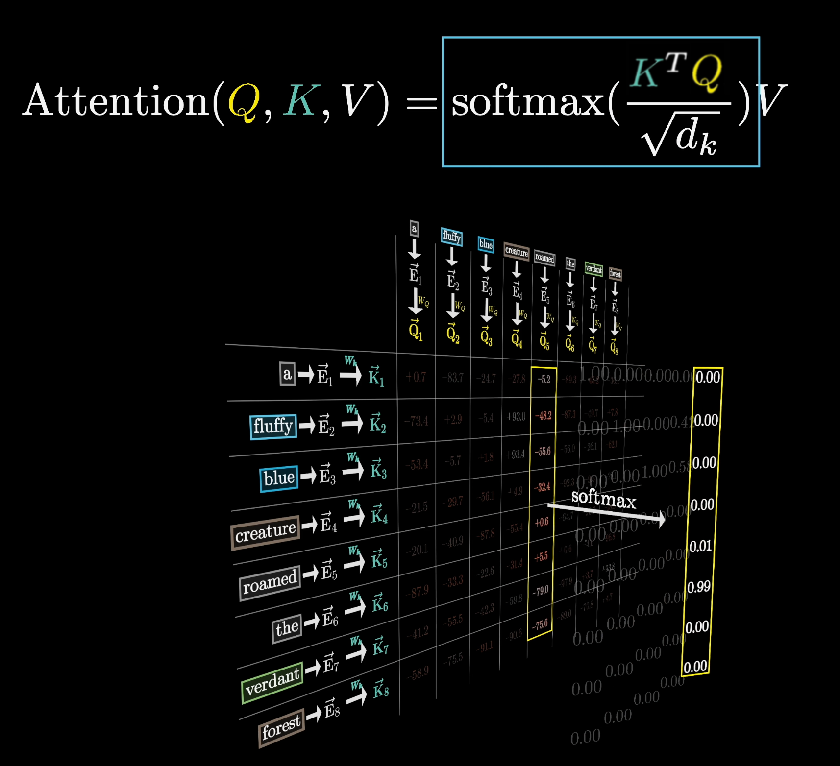
We want nonnegative attention weights that sum to 1 (a probability distribution), so we apply softmax along each column to normalize the scores.
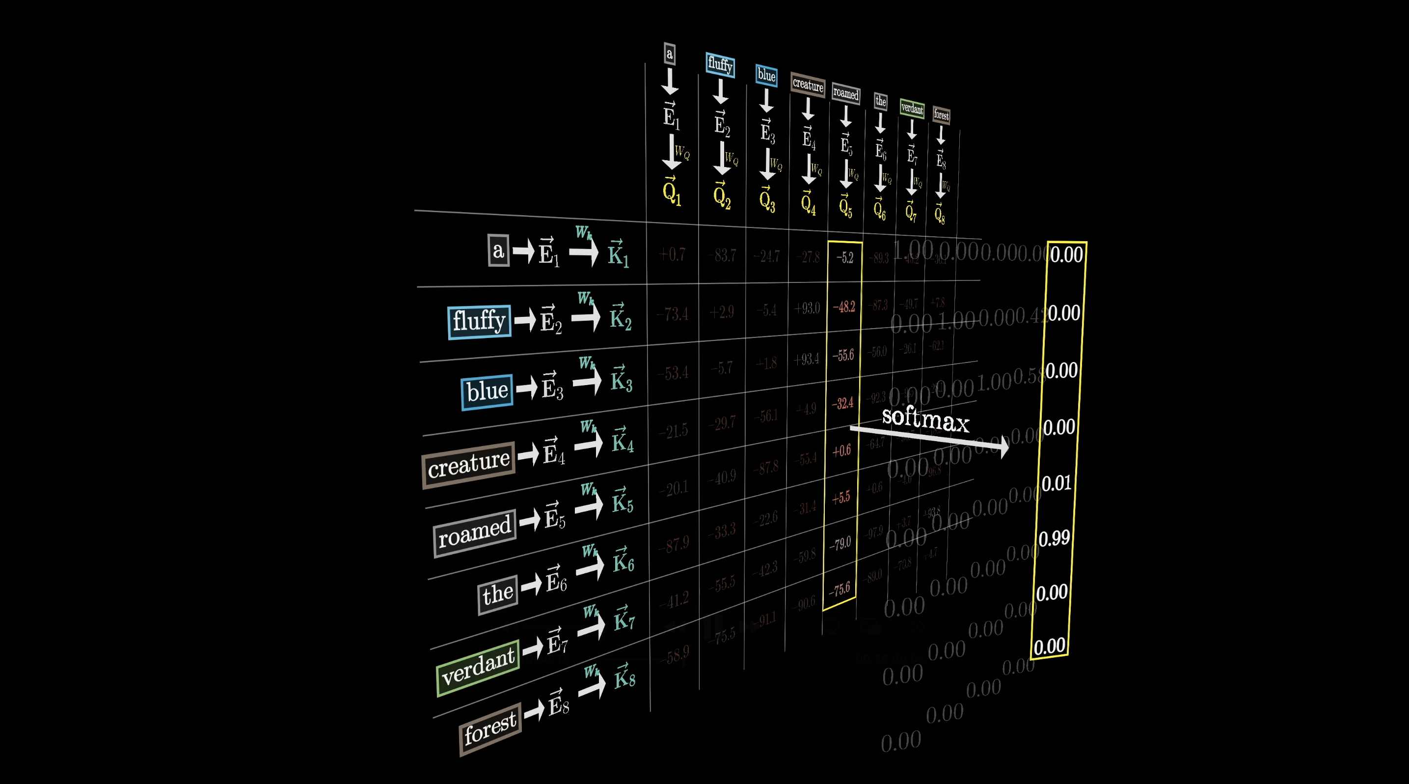
Softmax normalizes raw scores into attention weights
After softmax, the grid is filled with normalized values. This grid is the attention pattern.
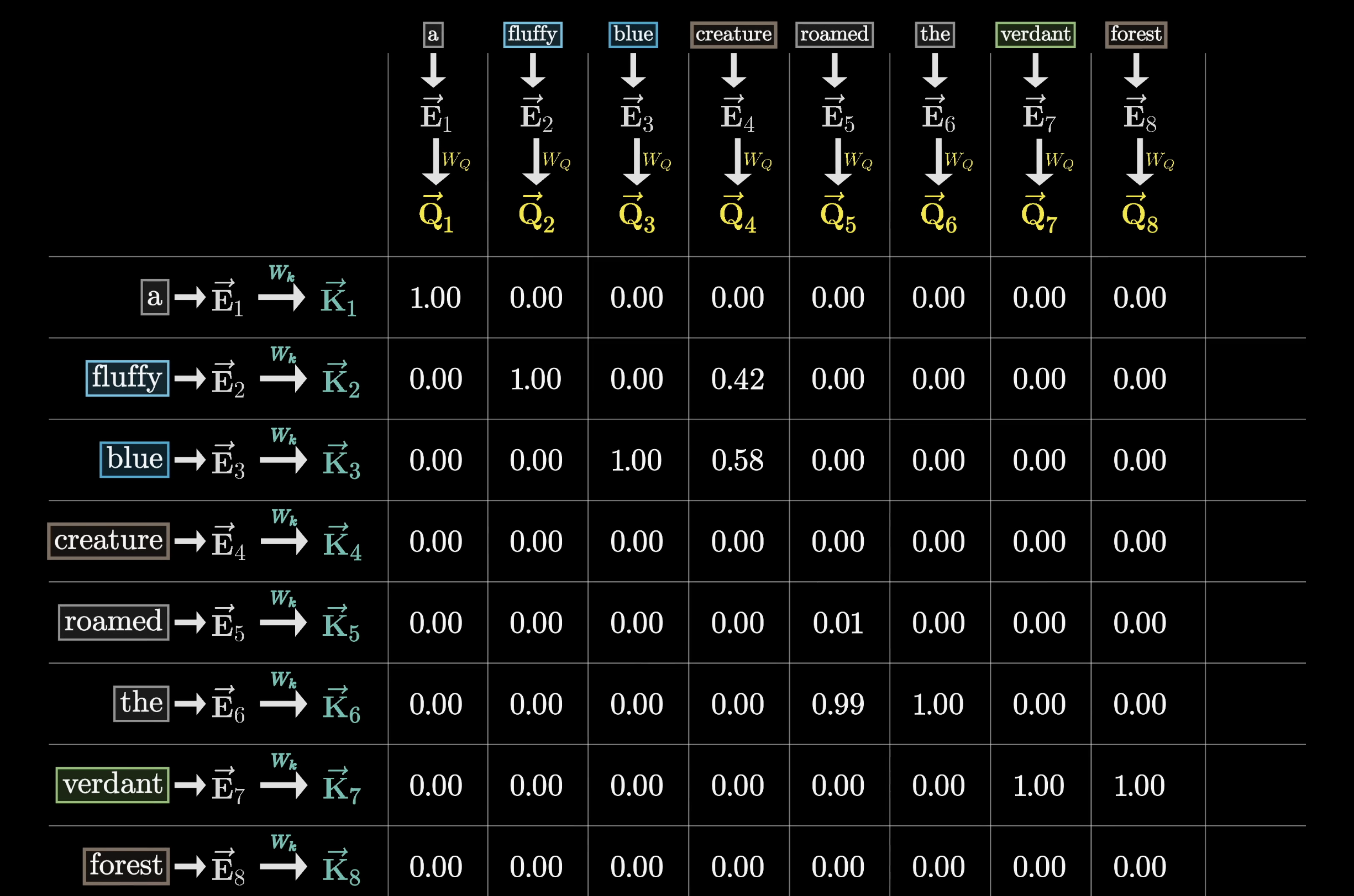
The attention pattern: each column is a probability distribution over positions
The Compact Formula
The original paper writes this compactly:
The scaled dot-product attention formula from the paper
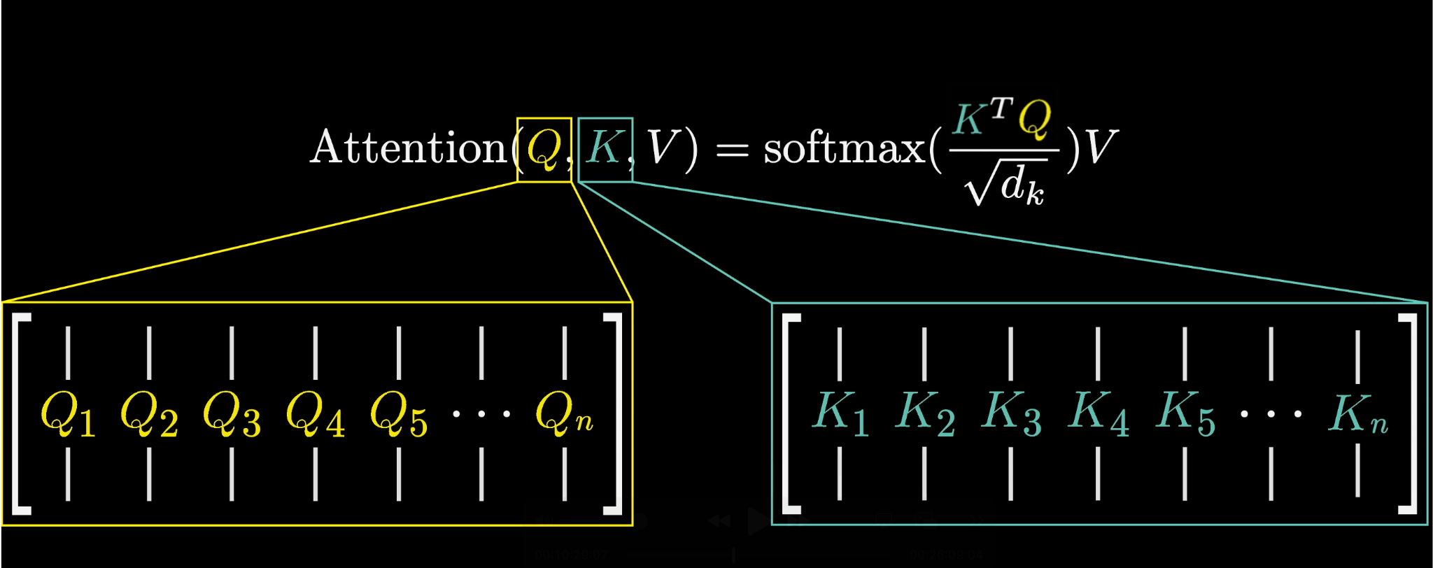
$Q$ and $K$ are the full arrays of query and key vectors. The product $K^T Q$ gives you the complete grid of dot products in one shot.
$K^T Q$ produces the complete score matrix in one operation
For numerical stability, the scores are scaled by $\sqrt{d_k}$ (the square root of the key-query dimension) before softmax.
Scaling by $\sqrt{d_k}$ keeps gradients well-behaved
Masking
During training, the model predicts every possible next token for every subsequence simultaneously. Much more efficient than doing them one at a time.
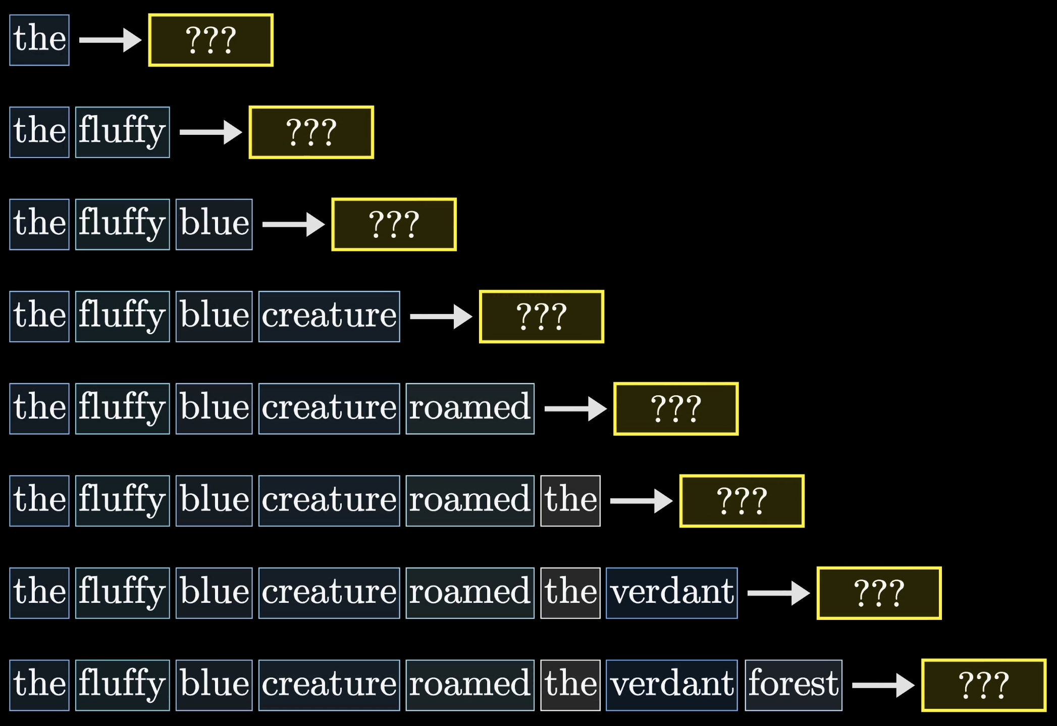
Efficient training: predicting every next token at once
But this means later tokens can never influence earlier ones, because that would give away the answer. So before softmax, we set the upper-triangle entries to $-\infty$, which softmax turns into zeros. This is called masking.
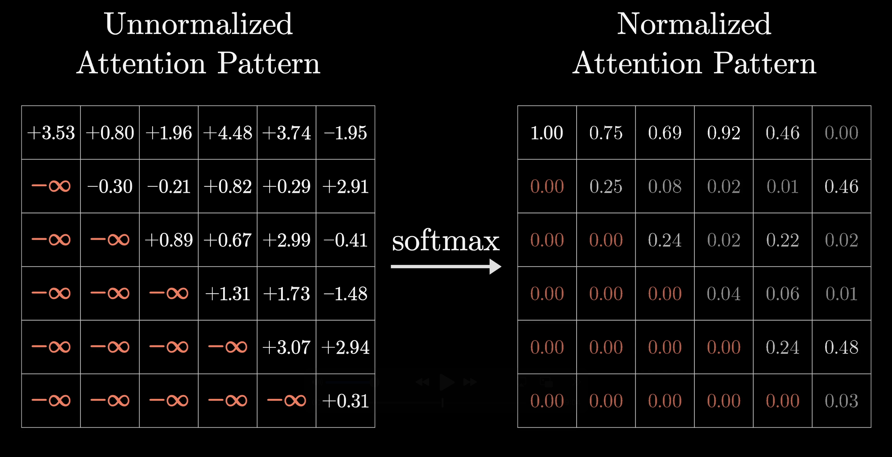
Masking prevents later tokens from influencing earlier ones
The attention pattern is $n \times n$ (one row and column per token), so it grows with the square of the context length. This is why scaling context windows is expensive, and why there's so much research into efficient attention.
Attention cost grows quadratically with context length
Values Carry the Information
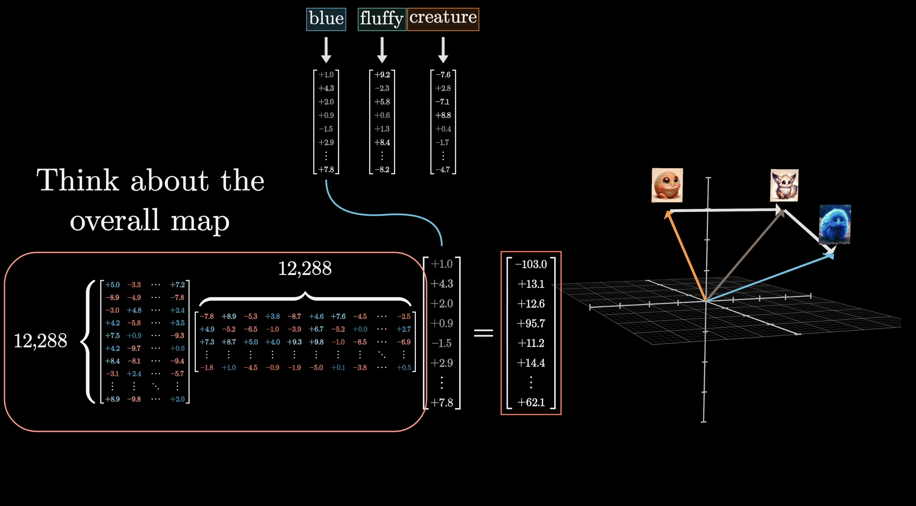
Keys decide where to look. Values decide what gets copied over. We want the embedding of "fluffy" to cause a change in "creature," moving it toward a region of embedding space that specifically encodes a fluffy creature.
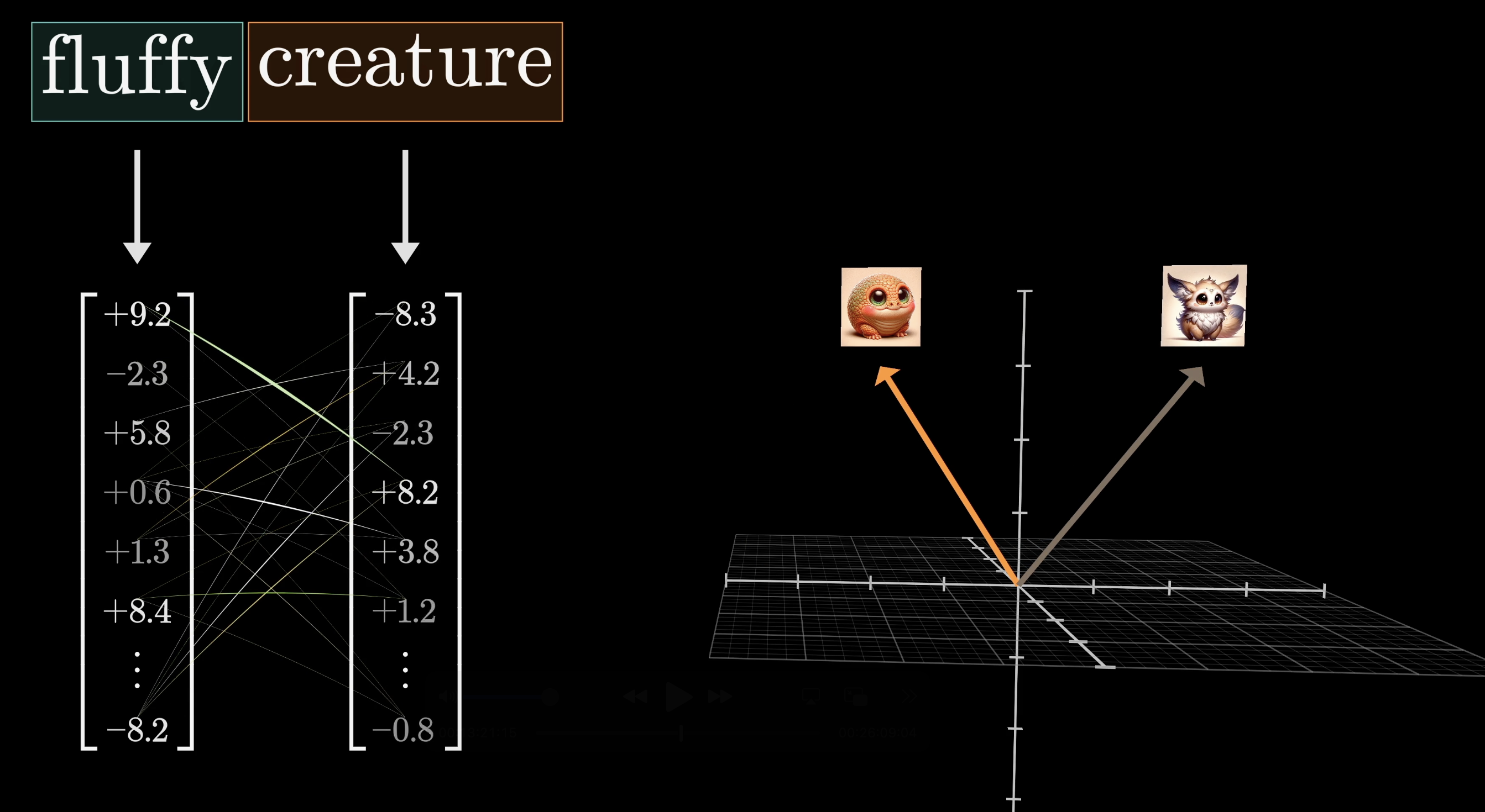
Values carry the actual information that updates embeddings
A third learned matrix, the value matrix $W_V$, maps each embedding to a value vector.
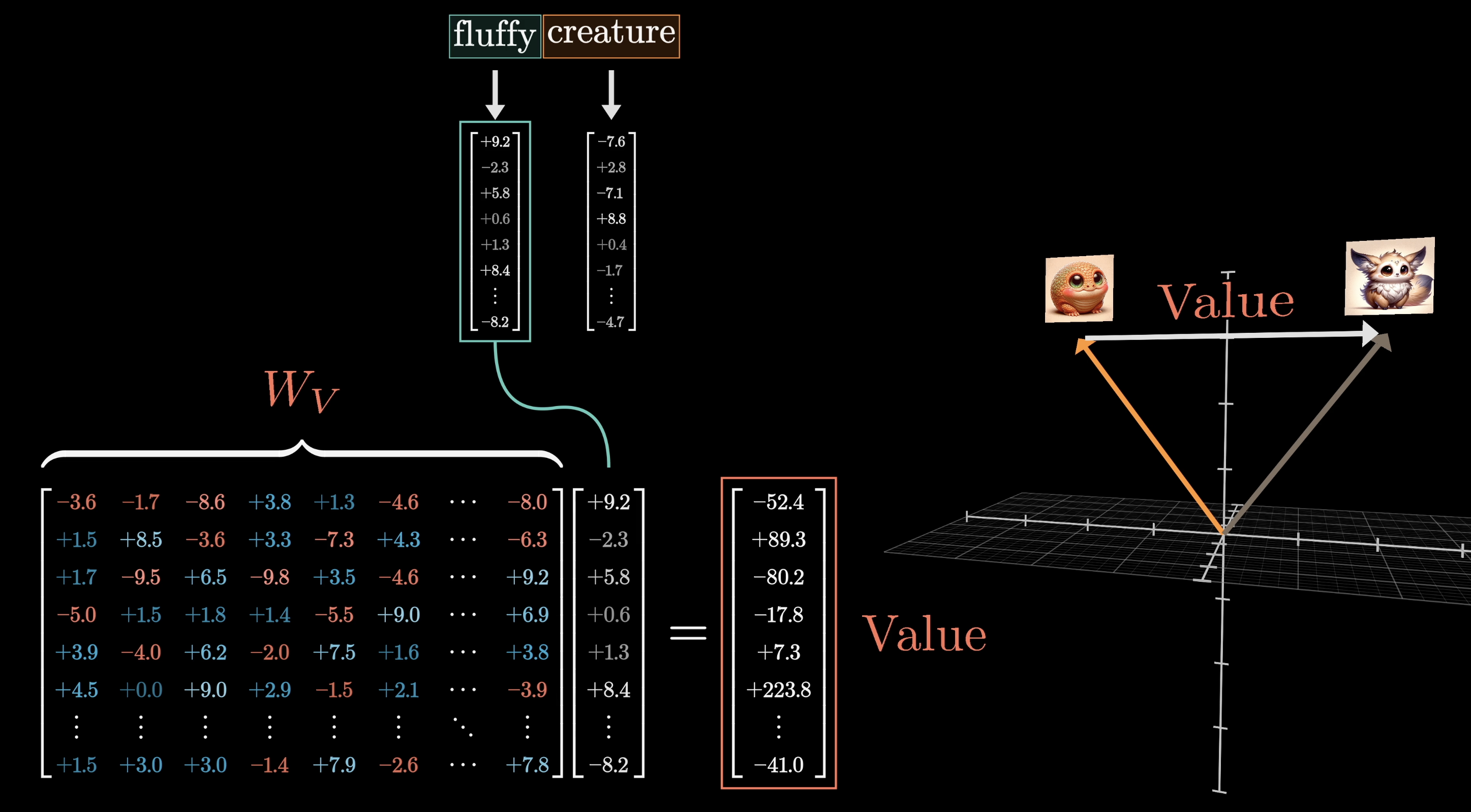
$W_V$ maps embeddings to transferable "content" vectors
For each column in the attention grid, we multiply each value vector by the corresponding weight.
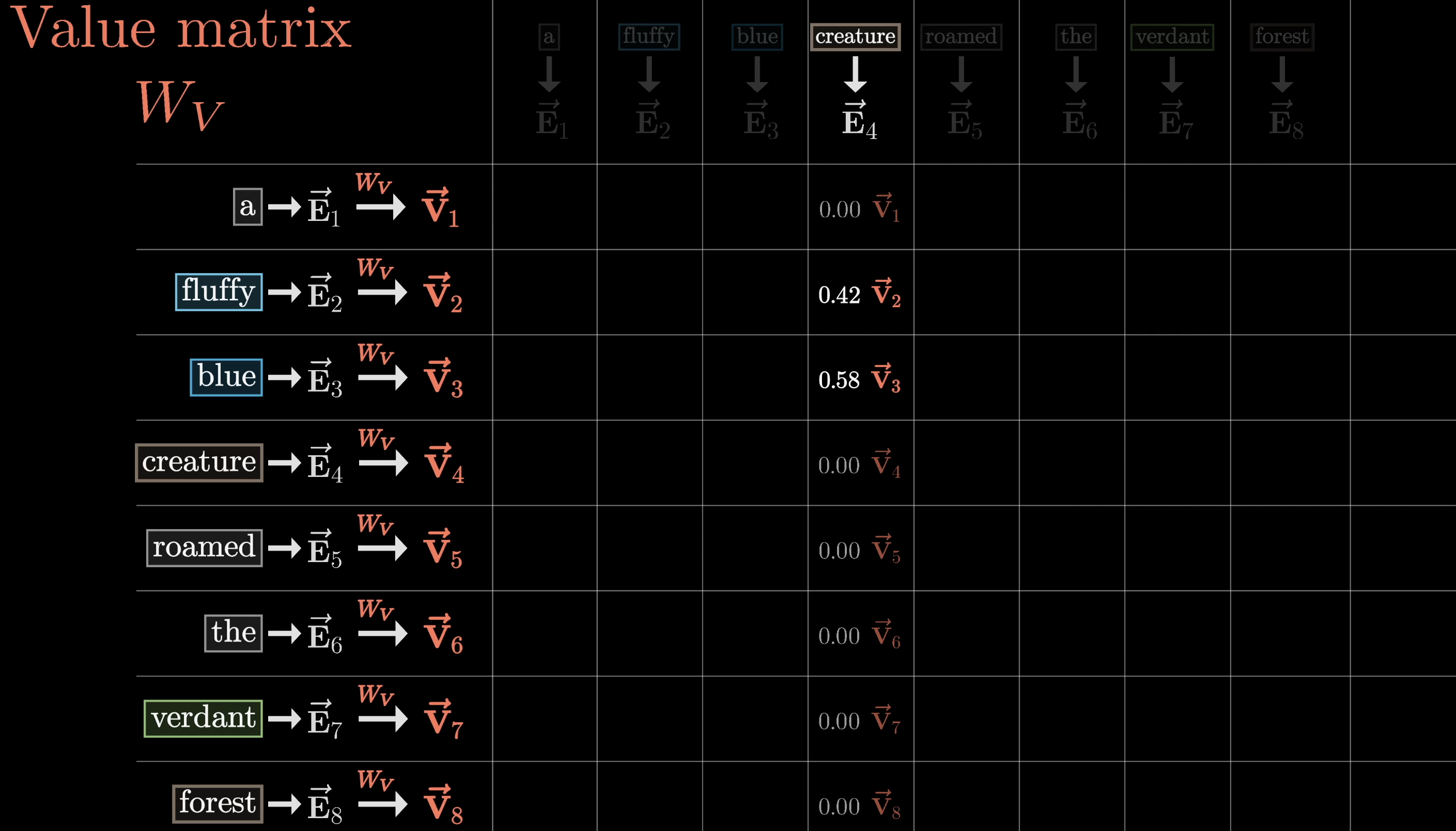
Weighted values: fluffy and blue contribute most under "creature"
Weighted Sum Builds the Update
Adding the rescaled value vectors in a weighted sum produces a change $\Delta \vec{E}$. Add that to the original embedding and you get a refined embedding $\vec{E}'$ that encodes richer, contextual meaning.
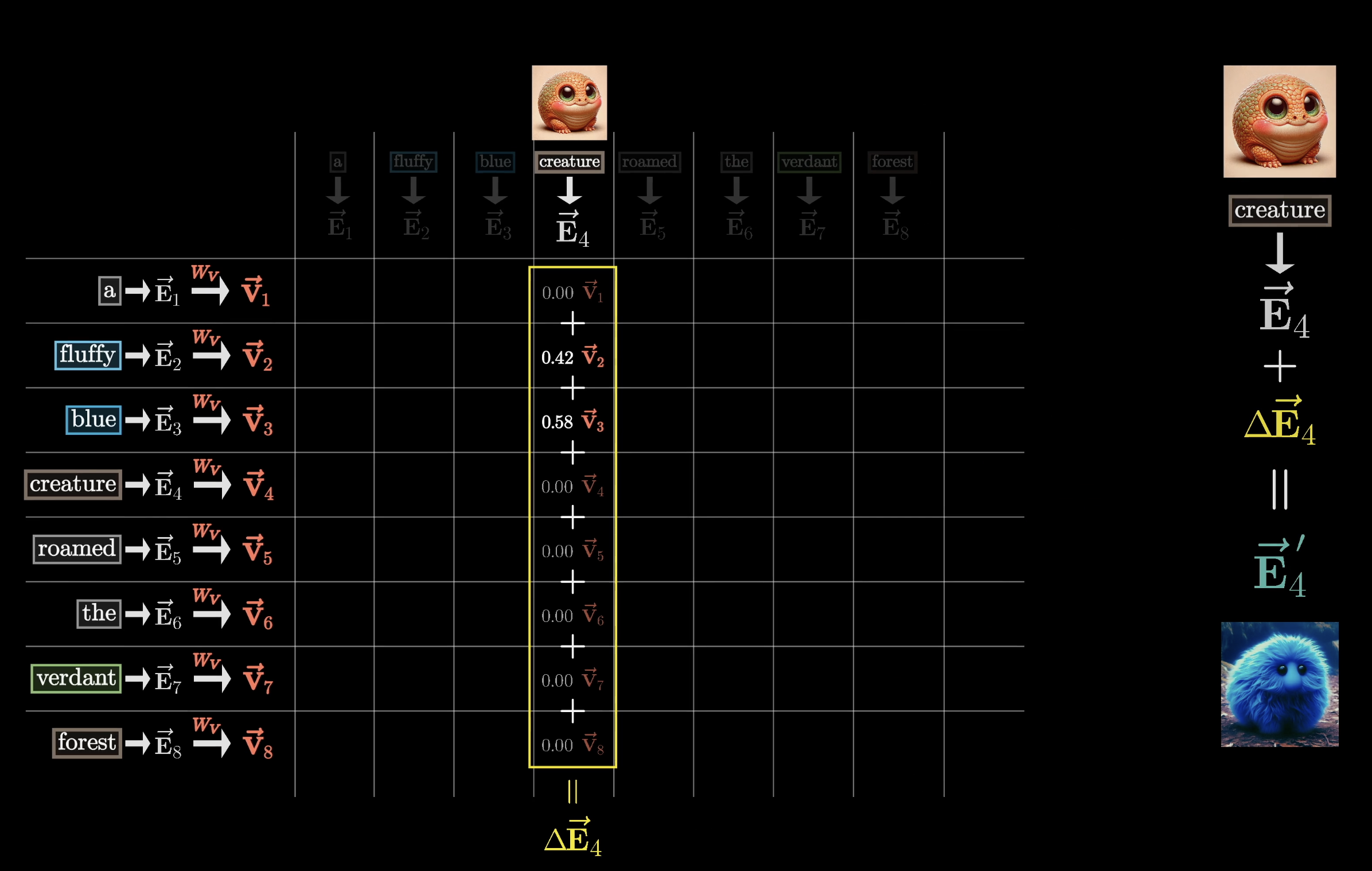
The weighted sum of values produces the update $\Delta \vec{E}$
This applies across all columns, producing a full sequence of refined embeddings out the other end. The whole process is a single head of attention, parameterized by three learned matrices: $W_Q$, $W_K$, and $W_V$.
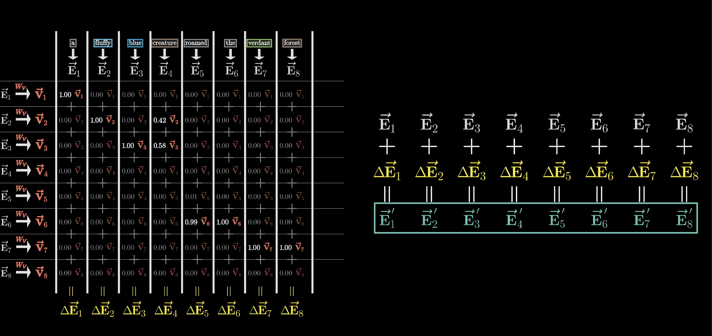
One attention head: $W_Q$, $W_K$, and $W_V$ together refine all embeddings
Counting Parameters
Using GPT-3's numbers: the key and query matrices each have 12,288 columns (the embedding dimension) and 128 rows (the key-query dimension), giving ~1.6M parameters per matrix.
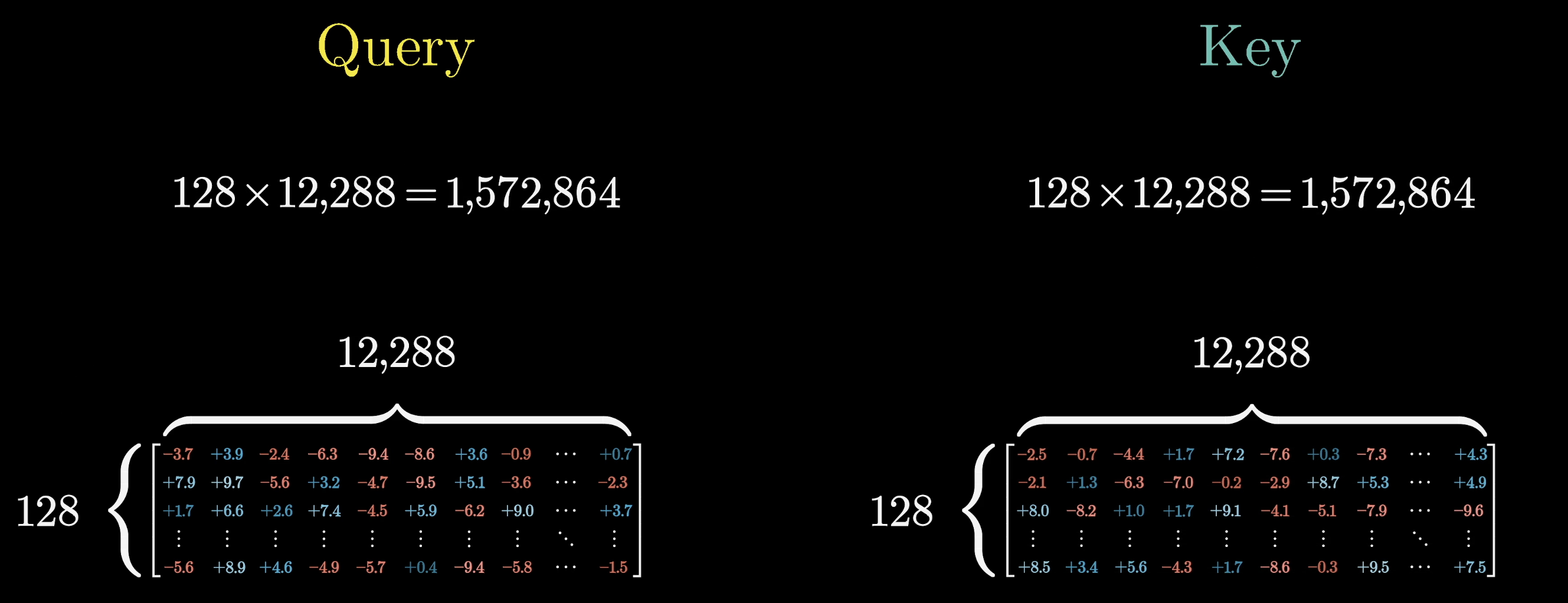
Query and key matrices: ~1.6M parameters each
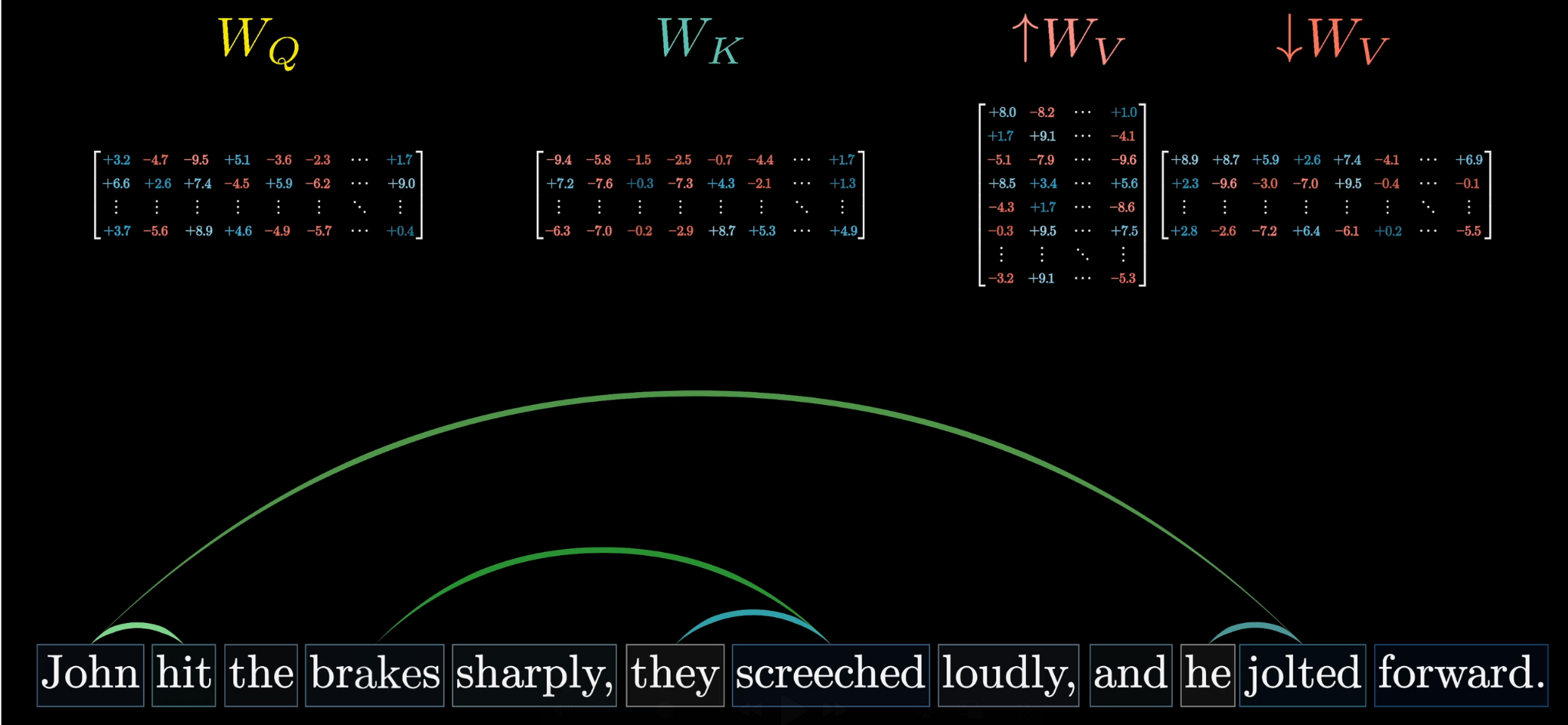
If the value matrix were a full $12{,}288 \times 12{,}288$ square, that would be ~151M parameters. Way too many. In practice, the value map is factored into two smaller matrices: one ($\text{Value}_\downarrow$) maps the embedding down to the 128-dimensional key-query space, and a second ($\text{Value}_\uparrow$) maps it back up. This makes it a low-rank transformation, keeping the parameter count balanced with the key and query matrices.
Keeping value parameters balanced with query/key parameters
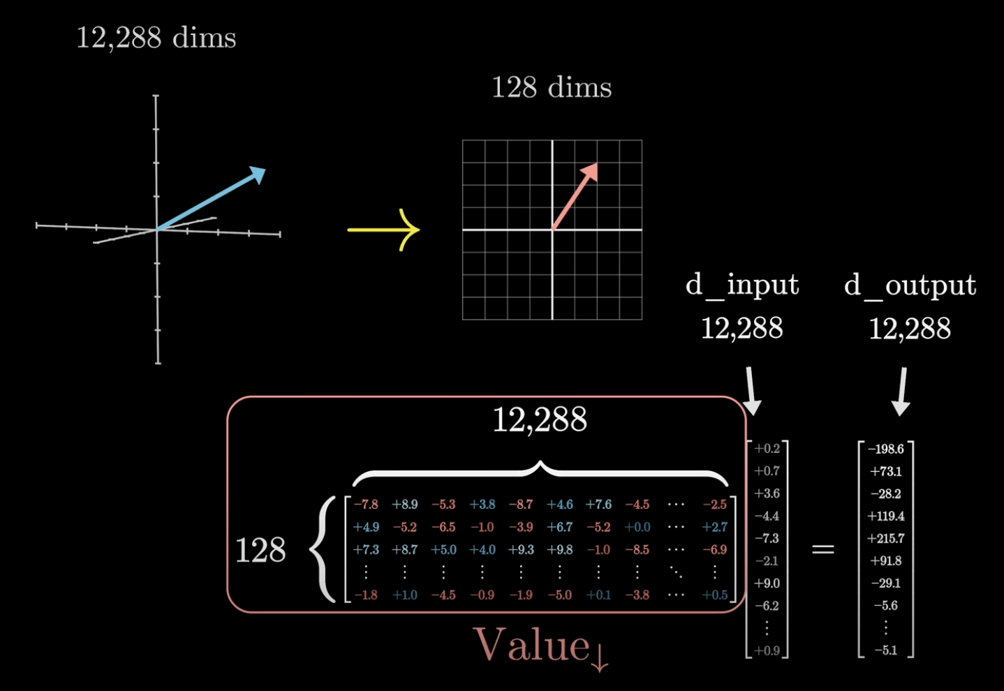
$\text{Value}_\downarrow$: embedding space down to key-query space
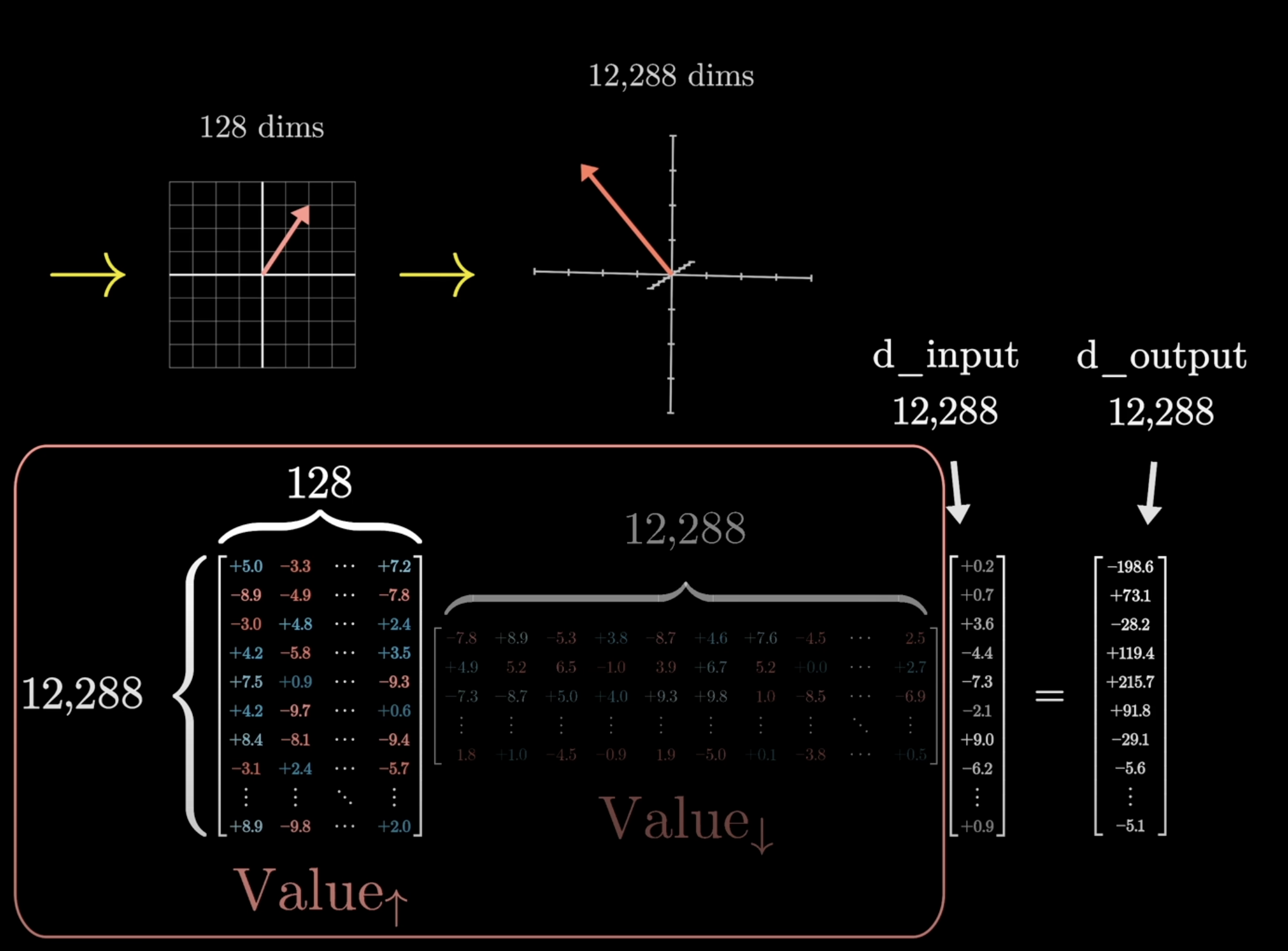
$\text{Value}_\uparrow$: key-query space back up to embedding space
All four matrices ($W_Q$, $W_K$, $\text{Value}_\downarrow$, $\text{Value}_\uparrow$) are the same size, totaling about 6.3 million parameters per head.
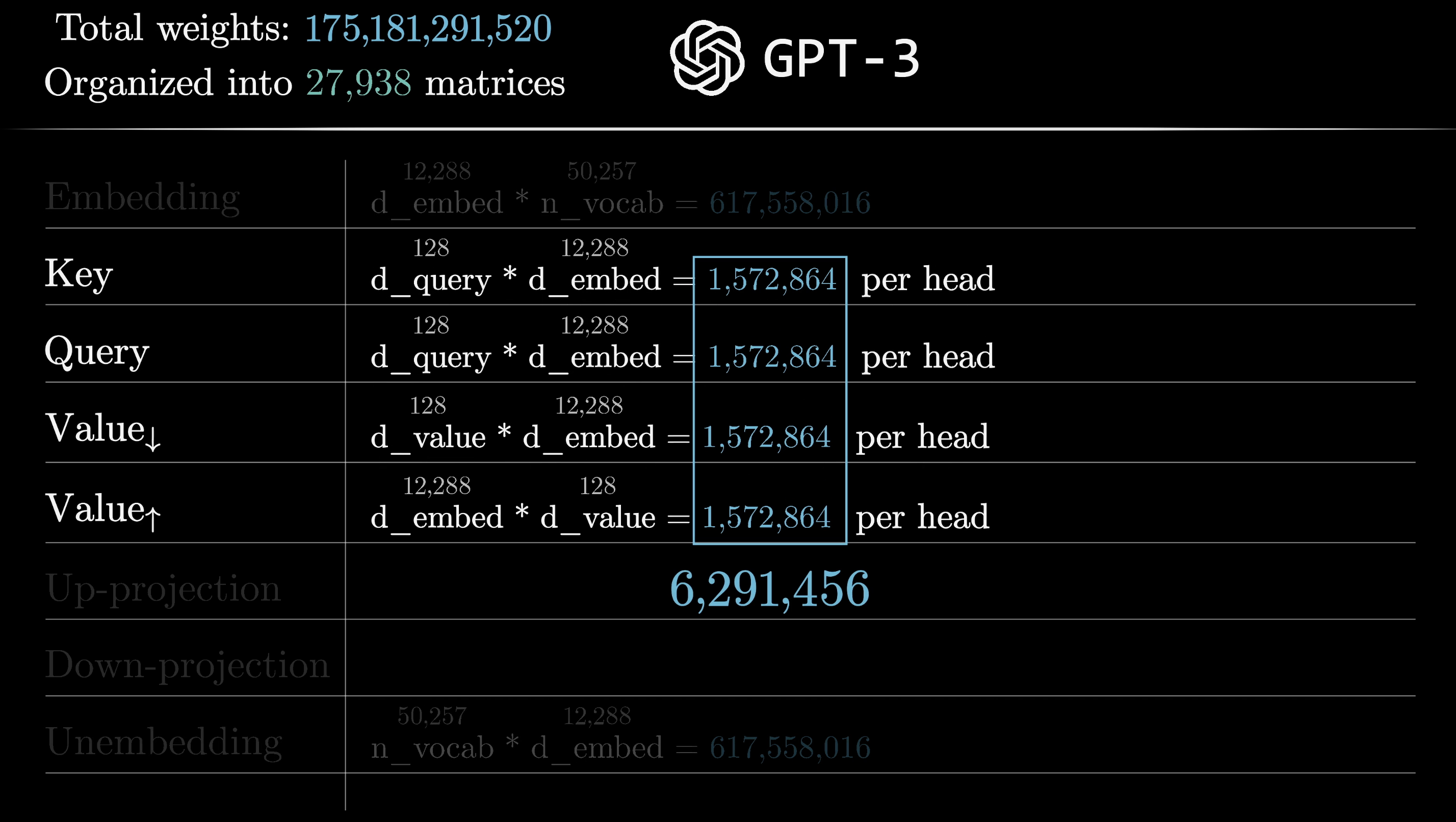
~6.3M parameters per attention head
Multi-Head Attention
A single head can learn one type of contextual interaction. But context influences meaning in lots of different ways. "They crashed the" before "car" has implications about the car's shape and condition. "Wizard" near "Harry" suggests Harry Potter, while "Queen" and "Sussex" suggest Prince Harry.
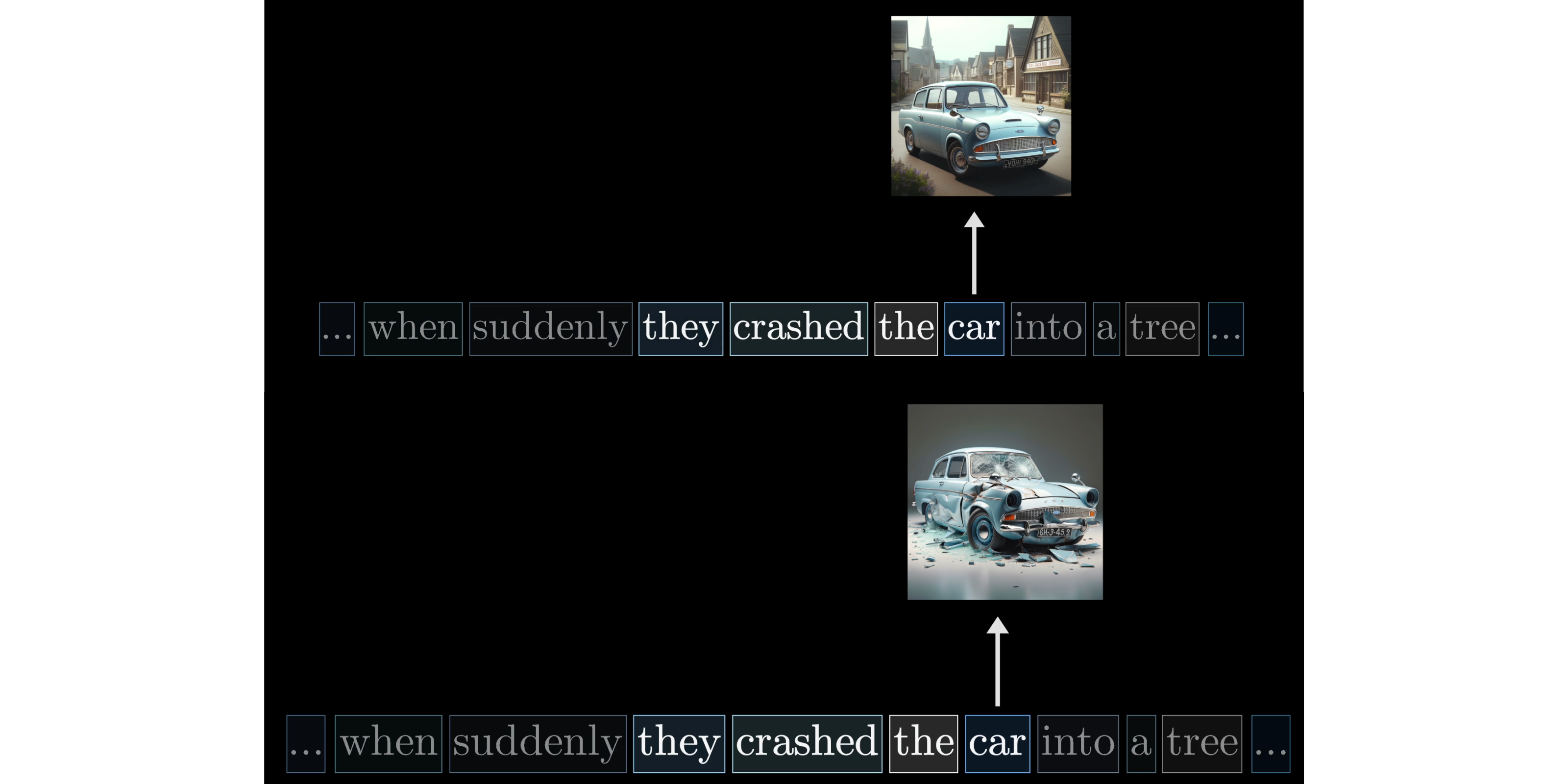
Different contexts call for different types of updates
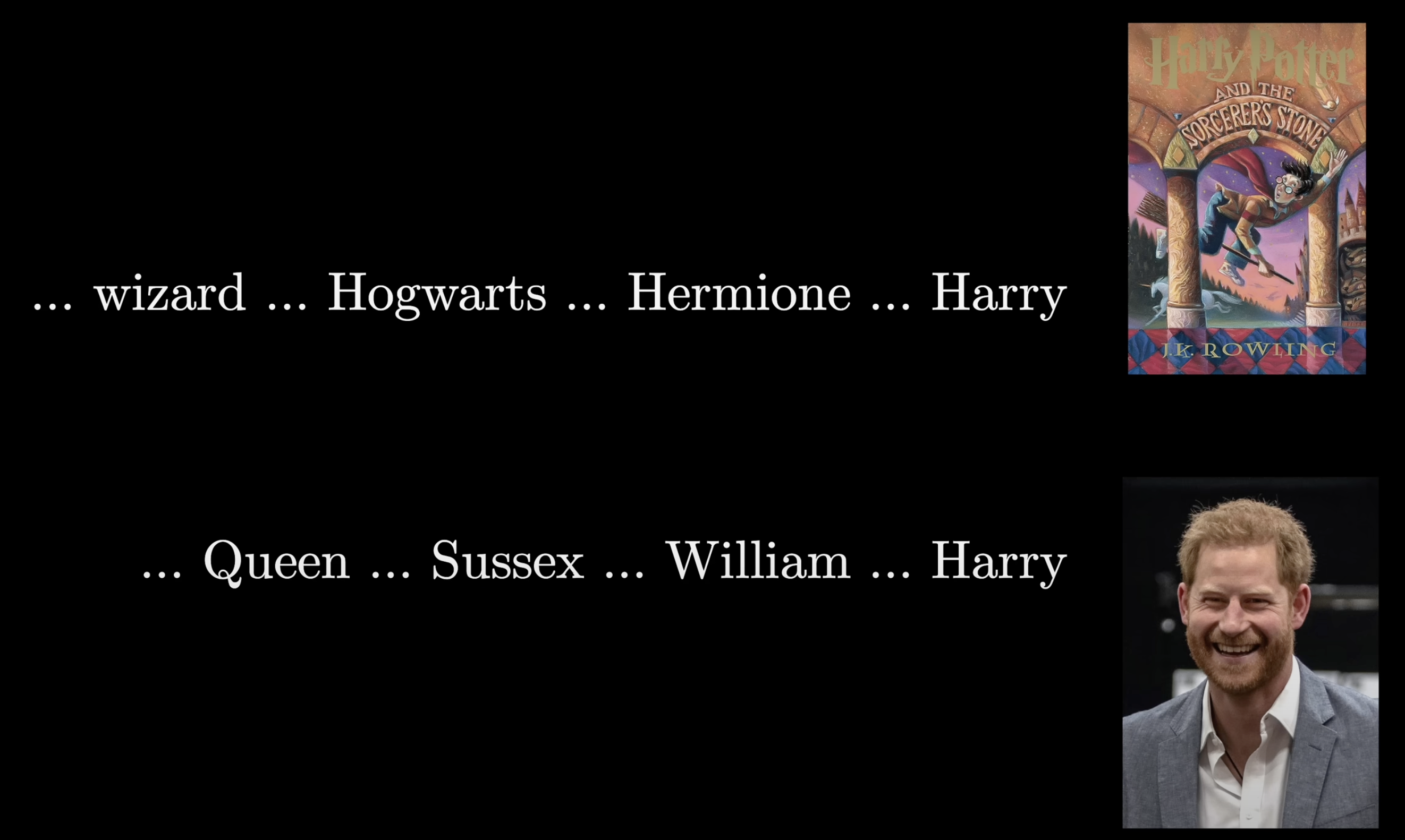
The same name can resolve to entirely different entities
Each type of contextual update needs its own $W_Q$, $W_K$, and $W_V$ matrices. A full attention block runs multi-headed attention: many heads in parallel, each with distinct parameters capturing different patterns. GPT-3 uses 96 attention heads per block.
Each head learns its own pattern of contextual interaction
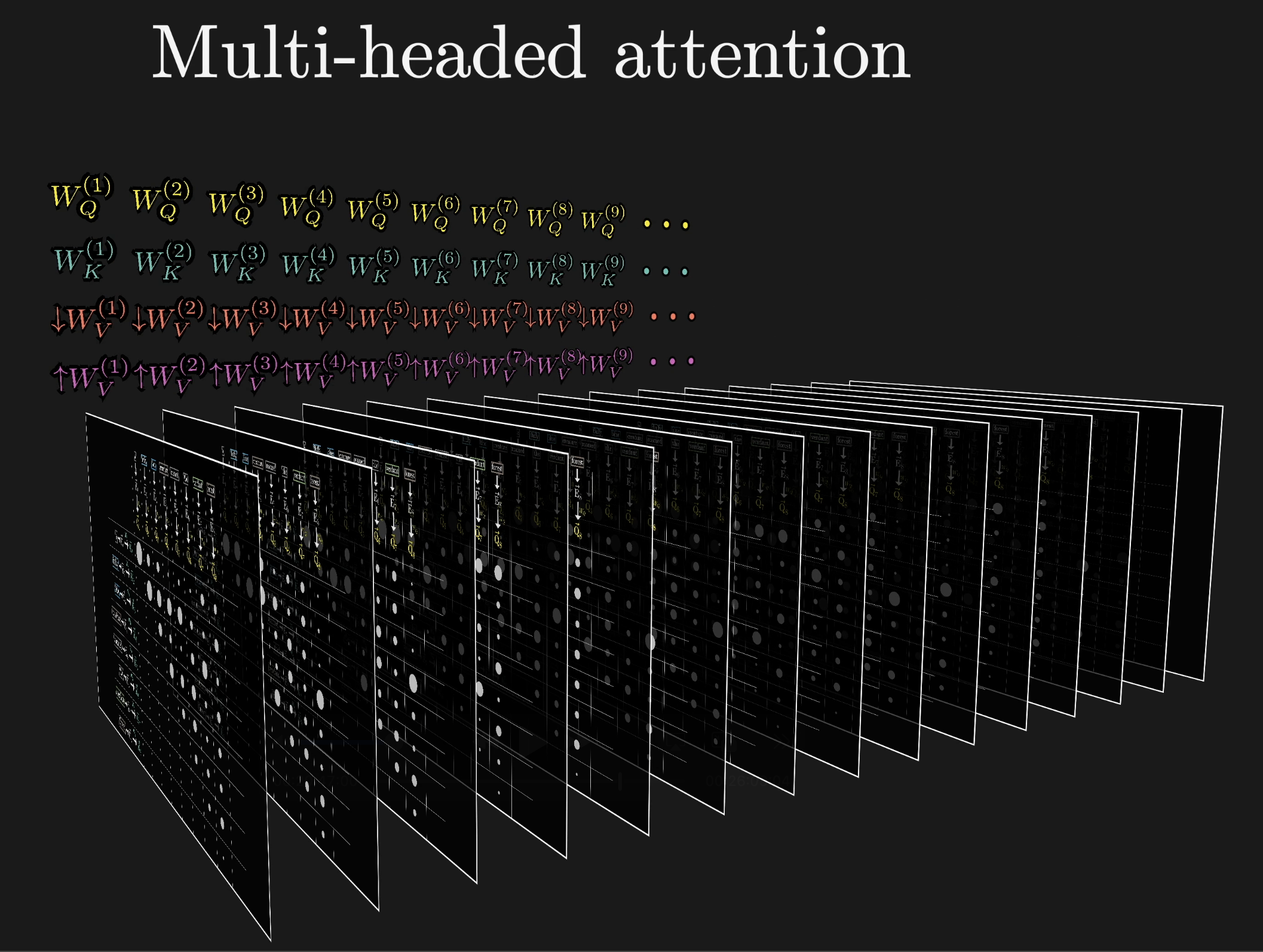
Multi-headed attention: many heads run in parallel
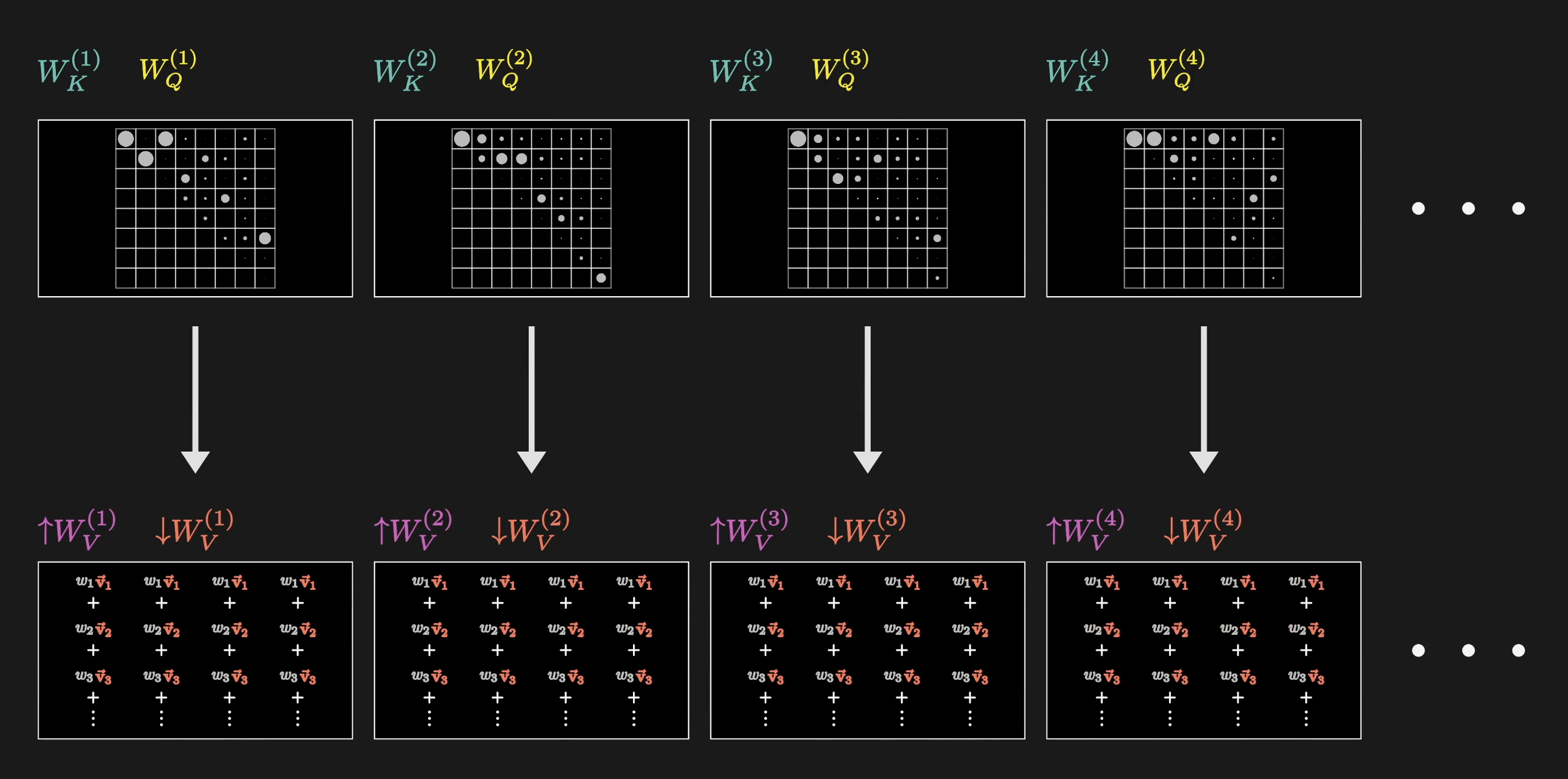
96 heads = 96 patterns, each capturing different contextual relationships
For each position, every head proposes a change $\Delta \vec{E}$. These all get added together and the result is added to the original embedding.
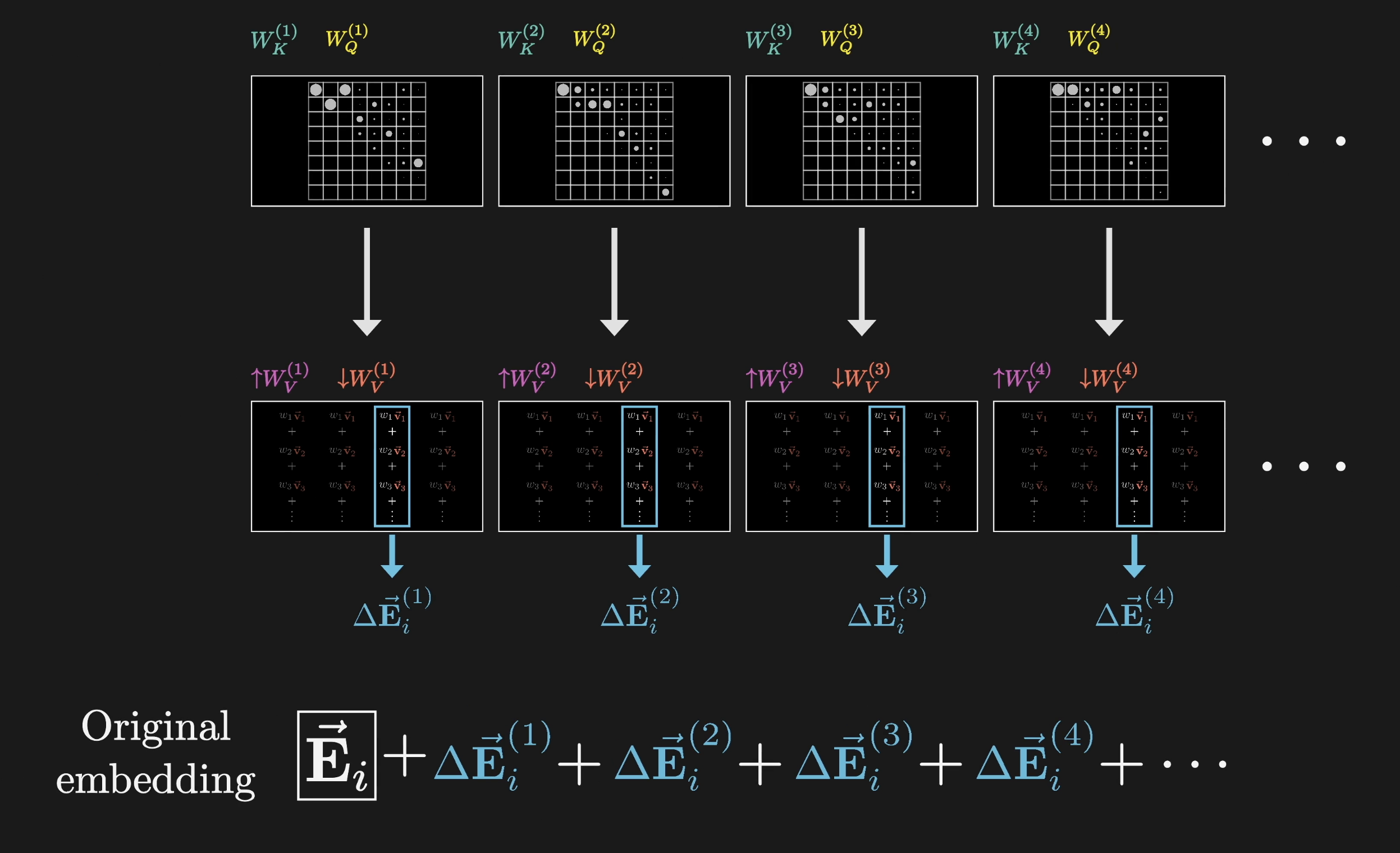
All heads contribute updates that are summed together
With 96 heads and four matrices each, a single multi-headed attention block has around 600 million parameters.
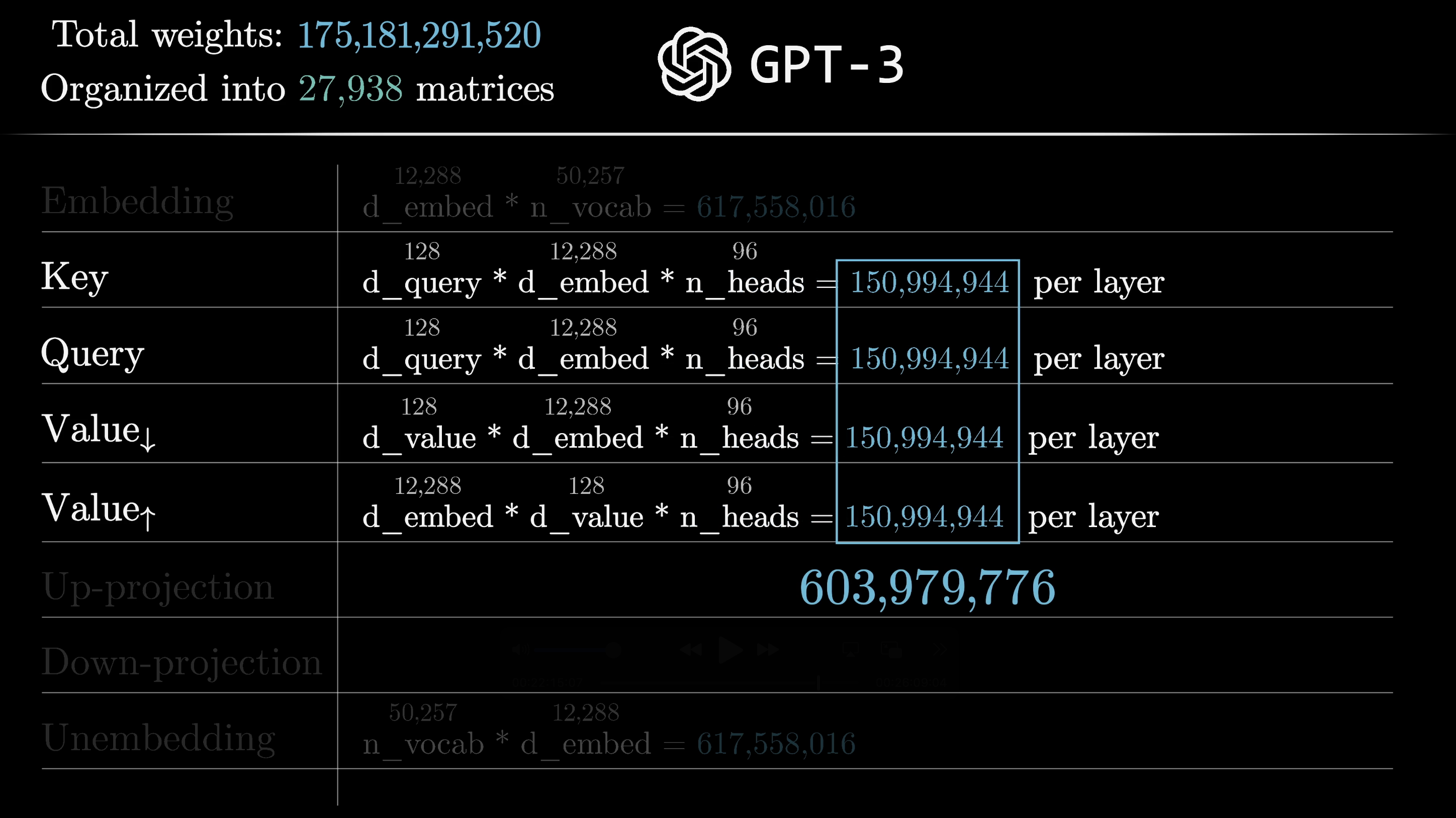
~600M parameters per attention block
Where This Sits in the Transformer
Data flowing through a transformer doesn't pass through just one attention block. It alternates between attention blocks and multi-layer perceptrons (MLPs), and this pair repeats many times across many layers.
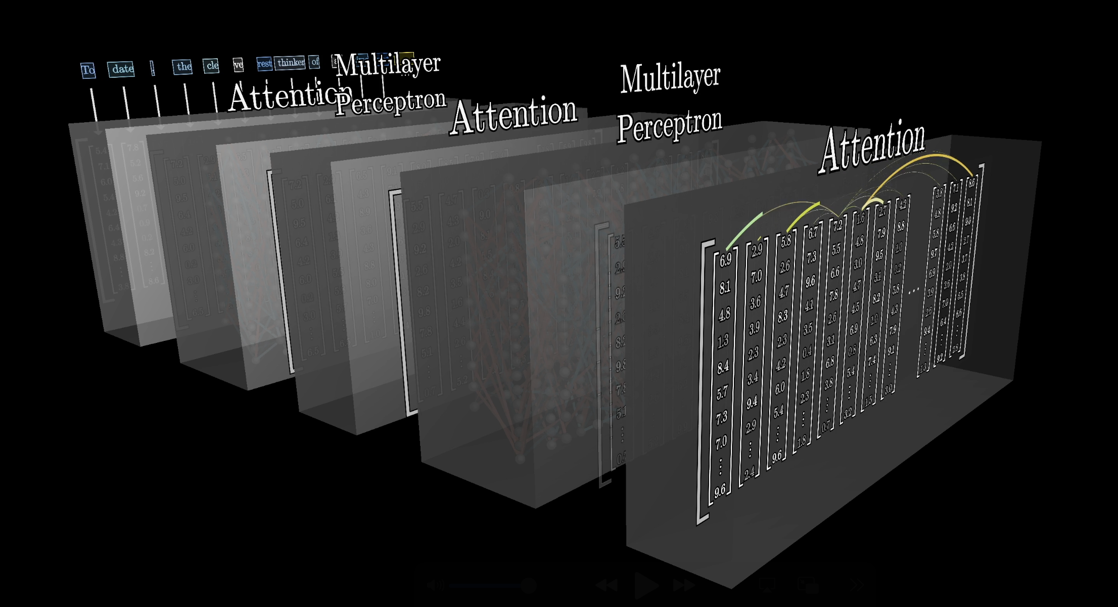
Attention blocks and MLPs alternate across many layers
The deeper you go, the more meaning each embedding absorbs from its (increasingly nuanced) neighbors. The hope is that deeper layers encode higher-level ideas: sentiment, tone, whether the text is a poem.
Depth enables increasingly abstract representations
GPT-3 has 96 layers, bringing the total attention parameter count to just under 58 billion. Sounds like a lot, but that's only about a third of the 175 billion total. The majority of parameters live in the MLP blocks.
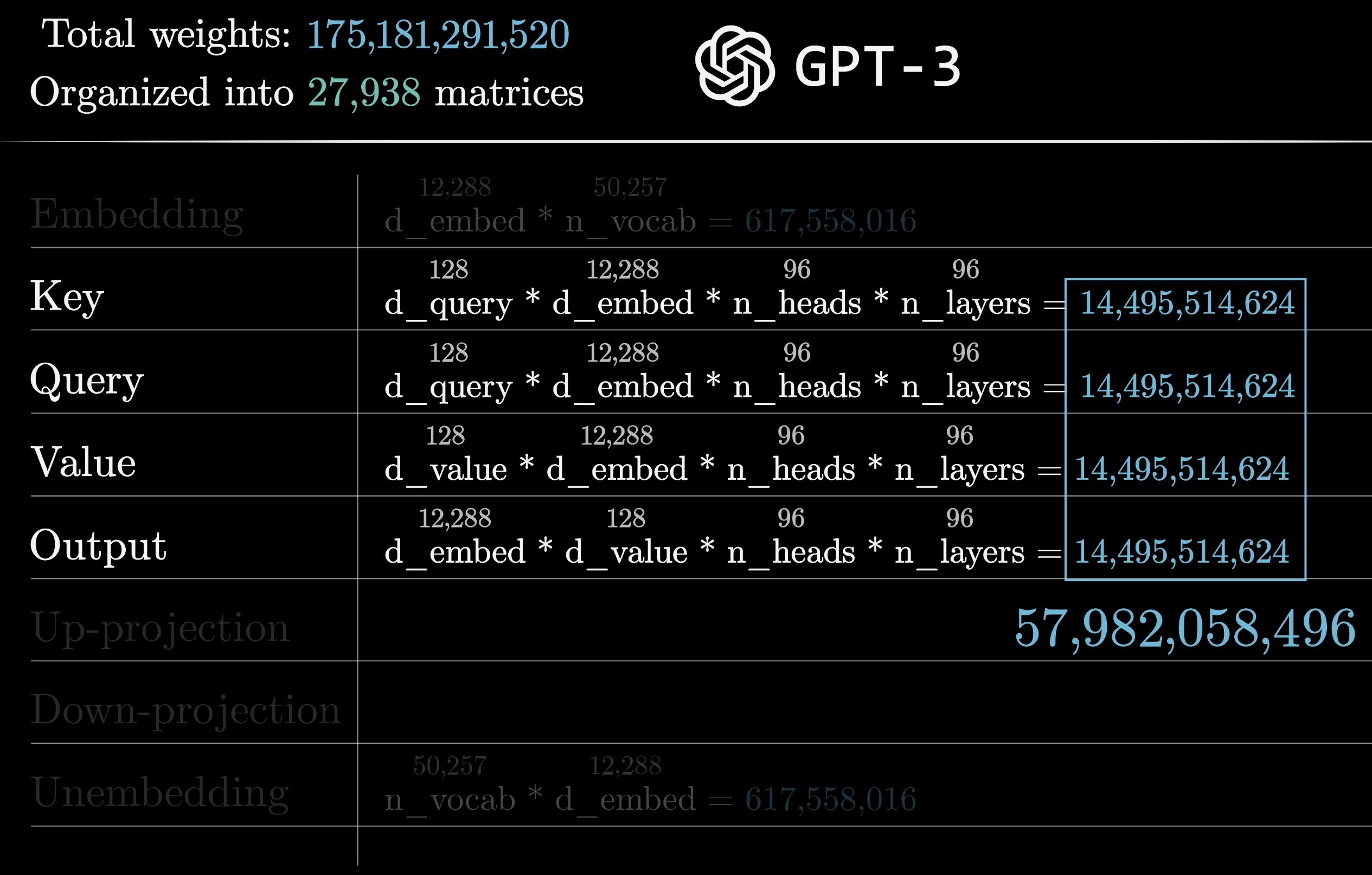
~58B attention parameters, roughly a third of GPT-3's total
A big part of attention's success isn't any specific behavior it enables. It's that the whole operation is massively parallelizable. It runs on GPUs incredibly efficiently, and scale alone has driven enormous improvements in what these models can do.
Summary
- Queries ($W_Q \vec{E}$): what this token is looking for
- Keys ($W_K \vec{E}$): what this token offers as a match
- Scores ($\vec{Q} \cdot \vec{K}$): relevance via dot products, scaled by $\sqrt{d_k}$
- Masking: prevents later tokens from influencing earlier ones
- Softmax: normalizes scores into attention weights
- Values ($W_V \vec{E}$): the information that gets mixed and copied
- Update: weighted sum of values → $\Delta \vec{E}$ → refined embeddings
- Multi-head: many heads learn many interaction patterns in parallel
- Depth: stacking layers lets embeddings absorb increasingly abstract context